Validity, Decoherence, and What Stochastic Gravity Does Not Capture

Stochastic gravity is reliable only for a typed observable in a typed approximation: a renormalized and smeared stress hierarchy, a stable causal response, weak physical metric fluctuations, and a declared large-N, loop, or cumulant order. Its classical random source can reproduce selected symmetrized correlations and describe decoherence of chosen histories, but it does not by itself specify a quantum metric state, measurement theory, or nonlinear spacetime superposition.

Required background. Large-N Quantum–Stochastic Correspondence fixes the strongest controlled quantum match; Higher Cumulants and Non-Gaussian Noise tests Gaussian closure; and Fixed Background, Semiclassical, EFT, and Quantum-Gravity Regimes fixes the regime handoff.

Helpful background. System–Environment Splits and Influence Functionals supplies the reduced-state meaning of noise, while Factorization Failure warns that a continuum region need not carry an autonomous tensor factor.

Conditions for a stochastic prediction

For a gauge-invariant smeared observable $Q[F]$, a useful set of dimensionless controls is

$$\epsilon_{\mathrm{EFT}} =\max\!\left( \frac{k_{\mathrm{phys}}}{\Lambda}, \frac{\sqrt{\lvert R\rvert}}{\Lambda} \right), \qquad \epsilon_{\mathrm{lin}} =\frac{\sqrt{\langle Q[F]^2\rangle_c}}{Q_{\mathrm{nl}}},$$

where $\Lambda$ is the low-energy cutoff, $k_{\mathrm{phys}}$ is the largest physical frequency or inverse sampling scale entering the response, and $Q_{\mathrm{nl}}$ is the scale at which nonlinear metric terms compete with the retained linear term. For a many-species construction also track

$$\epsilon_N=\frac{1}{N_f}, \qquad \gamma_3=\frac{\kappa_3[Q]}{\kappa_2[Q]^{3/2}}, \qquad \gamma_4=\frac{\kappa_4[Q]}{\kappa_2[Q]^2}.$$

A Gaussian leading large-N claim requires $\epsilon_{\mathrm{EFT}}\ll1$, $\epsilon_{\mathrm{lin}}\ll1$, a stable retarded response over the observation time, and standardized omitted cumulants smaller than the requested accuracy. It also requires a Hadamard or otherwise explicitly admissible matter state, finite smearing, fixed contact terms, solved constraints, and matching initial metric covariance. No one ratio replaces this collection.

The structure map should be read as a sequence of conditional reductions. Each arrow consumes assumptions and exports only the observable at its end.

A reproducible stochastic prediction states its stress hierarchy, response, smearing, gauge reduction, initial data, and controlled order before comparing with a quantum observable. The map is schematic and not to scale.

First application: assess a proposed curvature variance

Suppose a calculation claims a stochastic variance for a linearized curvature average over scale $\ell$ from $N_f$ identical scalar fields.

1. Distributional input. Verify that the state is Hadamard, the curvature sampler is smooth with finite support, and the composed stress sampler has characteristic scale $\ell$. Reject an unevaluated $N(x,x)$.
2. Cutoff separation. Require $\ell^{-1}$ and every response frequency to be well below $\Lambda$, and $\sqrt{\lvert R\rvert}\ll\Lambda$ on the causal domain.
3. Mean and response. Check that the background solves the renormalized mean equation and that the same finite local terms appear in the retarded operator. Physical homogeneous modes must remain bounded on the claimed interval.
4. Normalization. With $\mathbb E[\xi\xi]=N$, solve $\mathcal Lh=8\pi G\,\xi$ and verify the variance contains $(8\pi G)^2$.
5. Observable. Recompute the smeared curvature variance in a second gauge, including constraints and contact terms.
6. Closure. If only $N$ is retained, bound $\gamma_3$, $\gamma_4$, nonlinear response, and subleading $1/N_f$ corrections against the target uncertainty.

When these checks pass with $G=\bar G/N_f$, the strongest generic statement is

$$\mathbb E[Q[F]^2]_c =\frac12\left\langle \left\{\hat Q[F],\hat Q[F]\right\} \right\rangle_c +O(N_f^{-2})$$

for the declared linear gauge-invariant observable, assuming a regular expansion and matched intrinsic state. It is not a statement about an unsmeared metric, a commutator, or all quantum observables. The stability-and-fluctuation criterion underlying this conclusion is developed in Hu, Roura, and Verdaguer 2004, §§II–IV.

As of the evidence cutoff 10 August 2026, proposed local stress-fluctuation criteria remain prescription- and observable-sensitive. The OPE construction of Perez and Sudarsky 2026, eqs. (4)–(10) and (19) is a current result for suitable Hadamard states and specified renormalized products; it does not establish a universal pointwise breakdown threshold. A gravitational response can suppress or amplify a stress channel, so validity is decided at the requested metric observable.

Decoherence is a conditional statement

For two coarse-grained metric histories separated by $h_\Delta$, the quadratic influence functional contains

$$\left\lvert\mathcal F[h^+,h^-]\right\rvert =\exp\!\left[ -\frac12\,J_\Delta N J_\Delta \right], \qquad J_\Delta=-\frac12h_\Delta .$$

Large $J_\Delta N J_\Delta$ suppresses interference between those histories in the chosen reduced description. This is evidence of environment-induced decoherence for a specified system–environment split, initial state, coarse graining, and history basis Calzetta and Hu 1994, §§II–IV. It does not select one outcome, prove fundamental collapse, or turn every metric component into a classical observable. Different relational partitions can yield different reduced descriptions, and continuum local algebras need not factorize in the naive way.

The stochastic source is a representation of retained influence-functional cumulants. Its probability law is not automatically an ontic distribution of spacetime geometries. In particular, decoherence can be strong while the metric commutator or entanglement with inaccessible degrees of freedom remains essential.

Identical covariance does not mean identical information

Let a self-adjoint mode observable have four spectral values that support two diagonal states. State A assigns probabilities $1/2,1/2$ to values $-1,+1$. State B assigns probabilities $2/3,1/3$ to values $-1/\sqrt2,+\sqrt2$. Both have zero mean and unit variance, so a Gaussian stochastic model of that mode is identical for the two states. Their third moments are

$$\kappa_3^A=0, \qquad \kappa_3^B=\frac{1}{\sqrt2},$$

and their density-operator spectra—and therefore their von Neumann entropies—also differ. The covariance cannot determine higher moments, purity, entanglement, commutators, or distinguishability under other observables. The conclusion survives in field theory whenever the model retains only a finite set of smeared correlations.

Questions about the full quantum metric algebra, nonlinear superpositions, or complete information flow must be handed to Observable and Regime Matrix for Quantum Gravity. Generic reduced-dynamics and measurement constructions remain with Thermal and Nonequilibrium QFT.

Domain and failure conditions

Use the chapter comparison table to state the final claim ceiling. Downgrade the result if the sampler approaches a delta distribution, a physical response mode grows, the gauge comparison fails, the EFT scale is approached, omitted cumulants are uncontrolled, the large-N limit is nonuniform, or a symmetrized covariance is being used to answer an unsymmetrized or information-theoretic question.

The failure map summarizes these independent stopping conditions. Passing one branch never cancels failure of another.

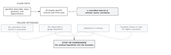
Stochastic gravity controls only the intersections of its distributional, dynamical, gauge, expansion, and information domains; outside that intersection the claim must be narrowed or transferred. The map is schematic and not to scale.

References

• Calzetta, E., and B. L. Hu. “Noise and Fluctuations in Semiclassical Gravity.” Physical Review D 49, 6636–6655 (1994). doi:10.1103/PhysRevD.49.6636. Open PDF
• Hu, B. L., A. Roura, and E. Verdaguer. “Induced Quantum Metric Fluctuations and the Validity of Semiclassical Gravity.” Physical Review D 70, 044002 (2004). doi:10.1103/PhysRevD.70.044002. Open PDF
• Perez, A., and D. Sudarsky. “Renormalization of the Quantum Stress Tensor Fluctuations and the Limits of Semiclassical Gravity.” Physical Review Letters, accepted 1 June 2026. doi:10.1103/jvj4-hk16. Open PDF