Einstein–Langevin Dynamics

The Einstein–Langevin equation propagates a stress covariance through the linearized causal semiclassical response. With the noise kernel normalized as $N=\frac12\langle\{t,t\}\rangle$, this chapter places $8\pi G$ on the stochastic source side. The induced metric covariance therefore carries $(8\pi G)^2$; the equation neither quantizes the metric nor includes graviton loops.

Required background. The Stress-Tensor Noise Kernel fixes the source covariance; Influence Functionals, Dissipation, and Noise derives its relation to the causal kernel; Linear Response, Stability, and Runaway Solutions supplies the deterministic operator; and Langevin Field Equations and Noise supplies the stochastic solution concept.

Helpful background. The Semiclassical Einstein Equation fixes the mean background, while Closed-Time-Path Generating Functionals in Practice fixes the in-in variation.

Linearized stochastic equation and normalization

Let the renormalized mean equation be

$$\mathcal E_{\mu\nu}[g] =8\pi G\,\langle\hat T_{\mu\nu}\rangle_g,$$

where $\mathcal E_{\mu\nu}$ includes the Einstein tensor, cosmological term, and the chosen local higher-curvature terms. The background $g$ is a solution. Define the causal linearized operator

$$\mathcal L_{\mu\nu}{}^{\alpha\beta}h_{\alpha\beta} \equiv \delta\mathcal E_{\mu\nu}[h] -8\pi G\,\delta\langle\hat T_{\mu\nu}\rangle[h],$$

where the second term contains the retarded stress response and its local contact terms. The Einstein–Langevin equation is

$$\boxed{ \mathcal L_{\mu\nu}{}^{\alpha\beta}h_{\alpha\beta}(x) =8\pi G\,\xi_{\mu\nu}(x) },$$

with

$$\mathbb E[\xi_{\mu\nu}(x)]=0, \qquad \mathbb E[\xi_{\mu\nu}(x)\xi_{\rho'\sigma'}(y)] =N_{\mu\nu\rho'\sigma'}(x,y).$$

An equally valid convention defines $\Xi_{\mu\nu}=8\pi G\,\xi_{\mu\nu}$. Then the equation reads $\mathcal Lh=\Xi$, but its covariance is

$$\mathbb E[\Xi_{\mu\nu}(x)\Xi_{\rho'\sigma'}(y)] =(8\pi G)^2N_{\mu\nu\rho'\sigma'}(x,y).$$

Using $\mathcal Lh=\Xi$ together with $\mathbb E[\Xi\Xi]=N$ would lose two powers of $8\pi G$ and is inconsistent with the mean equation.

The linearized Bianchi identity and the matter Ward identity require a conserved stochastic source. Distributionally,

$$\nabla^\mu N_{\mu\nu\rho'\sigma'}=0 =\nabla^{\rho'}N_{\mu\nu\rho'\sigma'},$$

so $\xi$ can be realized on the conserved test-tensor quotient. Initial data must also satisfy the linearized gravitational constraints; a formal solution of only the evolution equations is insufficient.

The structure map locates the equation after both kernels have been renormalized. Inspect the single causal arrow into the metric response: stochastic forcing does not replace the deterministic matter polarization.

Einstein–Langevin dynamics combines the retarded semiclassical operator with a zero-mean source of covariance $N$; its induced metric covariance consequently contains $(8\pi G)^2$. The map is schematic and not to scale.

Retarded solution and induced covariance

After gauge reduction and constraint solving, let $G^{\mathrm{ret}}$ be the retarded inverse on the physical linearized sector. With vanishing induced initial data,

$$h^{\mathrm{ind}}_{\mu\nu}(x) =8\pi G\int_M\mathrm dV_y\, G^{\mathrm{ret}}_{\mu\nu}{}^{\alpha'\beta'}(x,y) \xi_{\alpha'\beta'}(y).$$

Therefore

$$\begin{aligned} C^{\mathrm{ind}}_{\mu\nu\rho'\sigma'}(x,x') ={}&(8\pi G)^2 \int_{M^2}\mathrm dV_y\mathrm dV_z\, G^{\mathrm{ret}}_{\mu\nu}{}^{\alpha\beta}(x,y)\\ &\times N_{\alpha\beta\gamma'\delta'}(y,z) G^{\mathrm{ret}}_{\rho'\sigma'}{}^{\gamma'\delta'}(x',z). \end{aligned}$$

This expression is shorthand for a distributional pairing with external test tensors. It is finite only when the composed kernels and smearing define a valid pullback/product. The derivation and its influence-functional basis are given in Martín and Verdaguer 1999, §§III–IV and Hu and Verdaguer 2008, §§3.2 and 4.2.

First application: one gauge-invariant mode

Consider a gauge-invariant mode $Q_k(t)$ whose stable Markovian low-frequency equation is

$$\left(\partial_t^2+2\gamma_k\partial_t+\Omega_k^2\right)Q_k(t) =8\pi G\,\xi_k(t), \qquad \gamma_k>0,$$

and specify white noise only as a band-limited approximation,

$$\mathbb E[\xi_k(t)\xi_k(t')]=\mathcal N_k\delta(t-t').$$

The retarded Green function is

$$G_k^{\mathrm{ret}}(t) =\theta(t)e^{-\gamma_kt} \frac{\sin(\omega_kt)}{\omega_k}, \qquad \omega_k^2=\Omega_k^2-\gamma_k^2,$$

for the underdamped case. The late-time induced variance is

$$\begin{aligned} \mathbb E[Q_k^2] &=(8\pi G)^2\mathcal N_k \int_0^\infty\mathrm ds\, \left[G_k^{\mathrm{ret}}(s)\right]^2\\ &=\frac{(8\pi G)^2\mathcal N_k} {4\gamma_k\Omega_k^2}. \end{aligned}$$

The integral is positive, has the expected enhancement as damping tends to zero, and diverges when a stationary limit does not exist. In frequency space the general colored result is

$$C_k^{\mathrm{ind}}(\omega) =(8\pi G)^2 \left\lvert G_k^{\mathrm{ret}}(\omega)\right\rvert^2 N_k(\omega).$$

Thus a white approximation is licensed only over the response bandwidth; a quantum stress spectrum is generally colored and constrained by the fluctuation–dissipation relation only in a KMS state.

Adversarial consistency tests

If $\mathbb E[\xi]\ne0$, averaging the equation adds $8\pi G\,\mathbb E[\xi]$ to the already renormalized mean source. Unless that shift was deliberately removed from $\langle T\rangle$, it double counts the mean and fails to reduce to the causal semiclassical response equation.

If a proposed covariance has $N(f,f)<0$ for some real physical sampler, then the calculated metric variance is negative for a response concentrated in that direction. The source is not a real stochastic process. Finally, if $\mathcal L$ has an exponentially growing gauge-invariant homogeneous solution, finite noise does not establish stability; the chosen background fails the linear-response test independently of the induced variance.

Domain and failure conditions

The chapter comparison table licenses the result for linear perturbations about a self-consistent mean background, a causal renormalized response operator, conserved smeared noise, physical initial constraints, and a stated stochastic truncation. Intrinsic initial fluctuations are added on the next page. Nonlinear metric dynamics, graviton loops, unsymmetrized metric correlators, and a complete quantum state remain outside this equation.

The failure map identifies two common overclaims: omitting the dissipative kernel and calling the resulting classical covariance a full quantum metric state.

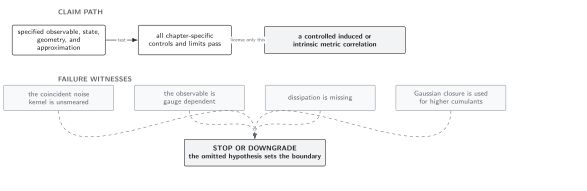
The equation controls a causal Gaussian-order metric covariance only when its mean, covariance, constraints, and $8\pi G$ factors match the influence functional. The map is schematic and not to scale.

References

• Hu, B. L., and E. Verdaguer. “Stochastic Gravity: Theory and Applications.” Living Reviews in Relativity 11, 3 (2008). doi:10.12942/lrr-2008-3. Open PDF
• Martín, R., and E. Verdaguer. “Stochastic Semiclassical Gravity.” Physical Review D 60, 084008 (1999). doi:10.1103/PhysRevD.60.084008. Open PDF