Total-Energy and Factorization Singularities

Cosmological boundary coefficients have energy singularities that remember bulk time evolution. A leading total-energy singularity can encode a flat-space amplitude, while partial-energy singularities encode on-shell propagation through a subgraph. These statements require a local tree interaction, a Bunch–Davies-type analytic branch, normalized external modes, and a specified continuation in complex energy space.

Required background. Contact and exchange seeds provide explicit coefficients, and the object dictionary fixes their normalization. Tree-level factorization supplies the amplitude comparison, while branches and monodromy supplies the complex-analysis language.

Helpful background. Analyticity and crossing of amplitudes explains the distinct flat-space sheet structure.

Total energy is a complex limit

For $n$ external modes, define

$$k_T=\sum_{a=1}^n k_a, \qquad k_a=\sqrt{\mathbf k_a^2}.$$

On the physical cosmological configuration $k_a>0$, so $k_T$ cannot vanish. The limit $k_T\to0$ is reached by analytic continuation of the complex energies, with every square-root and mode-function branch specified. For a local tree-level Bunch–Davies coefficient, the far-past portion of a contact integral has the form

$$\int_{-\infty(1-i\epsilon)}^0d\eta\, (-\eta)^q e^{ik_T\eta} \propto \frac{\Gamma(q+1)}{(ik_T)^{q+1}}.$$

The leading coefficient is determined by the corresponding early-time, approximately flat interaction. After stripping the known powers, external-mode normalizations, couplings, and continuation phase, it is the flat-space amplitude. The order of the singularity depends on $q$; “total-energy pole” does not always mean a simple pole.

The inference fails for a generic excited state because negative-frequency pieces produce additional signed energy sums, for nonlocal interactions because the early-time kernel need not be polynomial, and at loops because logarithms and multiparticle thresholds replace the simple tree structure.

A contact and exchange benchmark

For the conformal half-space contact seed,

$$\widehat\psi_4^{\mathrm{contact}} =\frac{\lambda}{k_T},$$

the reduced residue is

$$\operatorname*{Res}_{k_T=0} \widehat\psi_4^{\mathrm{contact}}=\lambda.$$

With an amplitude convention in which the stripped quartic contact amplitude is $\widehat{\mathcal A}_4=\lambda$, the two agree exactly. Restoring $i$ factors and external normalizations changes the dictionary but not this check.

An analytically controlled two-vertex scalar seed is

$$\widehat\psi_{4,s} =\frac{g^2}{k_T E_L E_R},$$

where

$$x_L=k_1+k_2,\quad x_R=k_3+k_4,\quad p=\lvert\mathbf k_1+\mathbf k_2\rvert,$$ $$E_L=x_L+p,\qquad E_R=x_R+p,\qquad k_T=x_L+x_R.$$

At total energy zero, $x_R=-x_L$, and

$$\operatorname*{Res}_{k_T=0}\widehat\psi_{4,s} =\frac{g^2}{p^2-x_L^2}.$$

Up to the declared overall sign, this is the flat $s$-channel propagator $g^2/(x_L^2-p^2)$. The sign is fixed by the branch and amplitude convention, not guessed from the rational function.

At the left partial-energy pole,

$$\operatorname*{Res}_{E_L=0}\widehat\psi_{4,s} =\left.\frac{g^2}{k_TE_R}\right|_{E_L=0},$$

which is the product of lower-point left and right data with the normalized internal kernel. For massive exchange, the pole can become a branch point and factorization is stated as a discontinuity. Baumann, Chen, Duaso Pueyo, Joyce, and Pimentel relate total- and partial-energy singularities to flat-space amplitudes and lower-point cosmological data (Baumann et al. 2022, §§ 2–4).

What remains invariant

Several operations have different effects:

• a bulk contact interaction changes the total-energy amplitude residue by the corresponding contact amplitude but does not change an exchange-channel residue;
• a local late-boundary counterterm adds an analytic polynomial and changes neither nonlocal residue;
• a local field redefinition redistributes bulk equation-of-motion and boundary contacts while preserving properly translated nonlocal data;
• a different analytic path on the same sheet gives the same residue;
• crossing a branch cut or encircling a branch point moves to a different sheet and must be reported.

The full boundary coefficient is therefore not fixed by its exchange singularities. Conversely, an arbitrary analytic addition cannot cancel a genuine nonanalytic exchange branch without violating locality or changing the spectrum.

Continuation-path adversarial test

Starting from $\widehat\psi_{4,s}$:

1. approach $k_T=0$ along two complex paths that remain on the same specified sheet;
2. approach $E_L=0$ while keeping $E_R$ nonsingular;
3. add an analytic boundary polynomial and a separate bulk quartic contact seed;
4. repeat after explicitly crossing the $p=\sqrt{(\mathbf k_1+\mathbf k_2)^2}$ branch cut.

The same-sheet total and partial residues must be path independent. The boundary polynomial changes neither. The bulk contact changes the total-energy residue by its flat contact amplitude but leaves the exchange residue fixed. The cross-cut value can differ and is labeled as another sheet. Any calculation that mixes these outcomes has not defined its analytic continuation.

The structure map separates total- and partial-energy information. Inspect how only the normalized leading total-energy coefficient reaches a flat amplitude, while partial energies factorize into lower cosmological objects.

Total-energy and exchange factorization data on specified complex sheets. The diagram is schematic and not to scale; locality, Bunch–Davies analyticity, normalization, and continuation path are required.

The failure map identifies overstatements. Inspect the stops for taking $k_T=0$ on the positive-energy locus, ignoring a branch sheet, or treating an analytic contact ambiguity as exchange data.

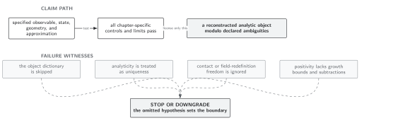
Failure conditions for amplitude extraction and factorization. The diagram is schematic and not to scale; a total-energy residue gives flat-space data only within the declared tree-level local standard-state domain.

These restrictions refine the chapter’s domain and failure conditions. Their unitarity content is developed in cosmological cutting identities.

Exercise

For $\widehat\psi_{4,s}=g^2/(k_TE_LE_R)$, compute its total-energy residue and verify that an added polynomial $c_0+c_1k_T$ does not change it.

Solution

Multiplying by $k_T$ and setting $x_R=-x_L$ gives

$$\operatorname*{Res}_{k_T=0}\widehat\psi_{4,s} =\frac{g^2}{(x_L+p)(-x_L+p)} =\frac{g^2}{p^2-x_L^2}.$$

For the polynomial,

$$\lim_{k_T\to0}k_T(c_0+c_1k_T)=0.$$

It therefore changes the analytic completion but not the residue.

References

• Baumann, D., W.-M. Chen, C. Duaso Pueyo, A. Joyce, and G. L. Pimentel. “Linking the Singularities of Cosmological Correlators.” Journal of High Energy Physics 2022, no. 09 (2022): 010. DOI. Open PDF.