Metastability, Eternal Inflation, and Claim Limits

A local vacuum-decay rate can determine the survival of a specified worldline or finite region. It cannot by itself assign probabilities to an infinite collection of inflating regions. Volume weighting adds a slicing and cutoff; stochastic self-reproduction adds a coarse-grained state and noise model; and extrapolation to arbitrarily long times adds semiclassical and quantum-gravity assumptions.

Required background. Coleman–De Luccia bounces and Hawking–Moss and stochastic crossing supply local transition candidates. Real-time state dependence fixes survival observables, and percolation and completion supplies the expanding-volume test.

Helpful background. The baryon-yield handoff and gravitational-wave propagation concern conditional observables inside completed histories. Gravitational EFT validity sets the semiclassical boundary.

Local decay and finite-region survival

Suppose a de Sitter-like false vacuum has constant $H$, a constant local decay rate $\Gamma$ per proper four-volume, and bubbles whose walls approach the speed of light. In a fixed finite comoving region, the false-vacuum probability is

$$P_F(t)=e^{-I(t)},$$ $$I(t)=\frac{4\pi\Gamma}{3H^3} \int_{t_i}^{t}dt'\, \left[1-e^{-H(t-t')}\right]^3.$$

At late times,

$$I(t)=\frac{4\pi\Gamma}{3H^3}t+O(1).$$

This controls a local or finite-region survival statement once the state and initial surface are fixed. A given timelike worldline is eventually struck with probability one in this idealized Poisson model because $P_F\to0$. No volume weighting is needed for that statement.

The expected physical false-vacuum volume associated with the same finite comoving region is instead

$$\langle V_F(t)\rangle \propto a(t)^3P_F(t) \sim \exp\!\left[ \left(3H-\frac{4\pi\Gamma}{3H^3}\right)t \right].$$

It grows on this flat slicing when

$$\frac{\Gamma}{H^4}<\frac{9}{4\pi}.$$

The simultaneous facts “each comoving worldline decays with probability one” and “expected false volume grows” are not contradictory. Expansion continually creates more physical volume from the surviving set. Guth reviews this distinction in false-vacuum eternal inflation (Guth 2007, §§ 2–3).

The numerical threshold is not universal. It assumes constant $H$ and $\Gamma$, luminal walls, homogeneous Poisson nucleation, a flat slicing, and an expectation value rather than a typical-volume statistic. A changing rate, collisions, terminal crunches, or another volume definition requires a new calculation.

Stochastic self-reproduction is another model

For a slowly rolling coarse-grained scalar, the fluctuation accumulated in one Hubble time is often estimated as

$$\delta\phi_q\simeq\frac{H}{2\pi},$$

while the classical drift is

$$\delta\phi_{\mathrm{cl}} \simeq\frac{\lvert\dot\phi\rvert}{H} \simeq\frac{\lvert V_{,\phi}\rvert}{3H^2}.$$

The inequality $\delta\phi_q\gtrsim\delta\phi_{\mathrm{cl}}$ diagnoses a diffusion-dominated regime in a particular Hubble-scale coarse graining. It does not by itself prove a global eternally inflating spacetime. The noise amplitude assumes a de Sitter-like prepared state and light field; the Fokker–Planck equation assumes a Markovian separation; volume weighting changes the evolution equation; and absorbing or reflecting boundaries change first-passage results. Vilenkin’s original diffusion picture already distinguishes local fluctuations from the reproduction of inflating domains (Vilenkin 1983, §§ II–III).

CDL, Hawking–Moss, and stochastic descriptions can all appear in one potential, but their rates and probability objects must be matched before comparison. A Hawking–Moss exponent is not automatically the transition kernel of a volume-weighted stochastic equation.

Cutoffs, time variables, and probabilities

An inflating spacetime can generate unbounded physical volume and infinitely many events. Relative frequencies then require a regulator. A global prescription must specify:

$$\text{time variable},\quad \text{cutoff hypersurfaces},\quad \text{initial distribution},\quad \text{vacuum transitions},\quad \text{observer or event weighting}.$$

Proper-time and scale-factor cutoffs truncate the spacetime on different hypersurfaces and can weight rapidly expanding or young regions differently. A monotonic reparameterization of a fixed finite-region integral cannot change its value; changing the cutoff surfaces of an infinite ensemble can change the regulated ratio. That is additional model data, not a coordinate paradox. Freivogel reviews how multiverse predictions inherit this measure dependence (Freivogel 2011, §§ 2–4).

This page therefore makes no measure-independent claim that one vacuum, observation, or cosmological history is probable. It licenses only conditional statements of the form: given this coarse graining, state, transition kernel, time variable, and cutoff, the regulated statistic is …

Adversarial measure test

First compute $P_F$ and $a^3P_F$ for a finite comoving region using cosmic time $t$ and e-fold time $N=Ht$. With the same physical endpoints, the answers must agree and the sign of $d\log(a^3P_F)/dt$ is unchanged.

Next construct a two-vacuum branching model with different Hubble rates and terminal decay channels. Truncate once at fixed proper time and once at fixed scale-factor time, using the same initial patch and transition matrix. If the regulated event ratios differ, report both and identify the cutoff. Do not average them into a purported invariant probability.

Finally vary the stochastic coarse-graining scale and the initial density matrix within their controlled range. A conclusion that disappears under these variations is a model-dependent diffusion result, not a robust global theorem.

Semiclassical boundary

Define the invariant curvature scale

$$\mathcal K_R \equiv \left\lvert R_{\mu\nu\rho\sigma}R^{\mu\nu\rho\sigma} \right\rvert^{1/4},$$

supplemented by the corresponding Ricci invariants when they contain independent scales. Every long-time extrapolation must retain the hierarchy

$$H,\quad \mathcal K_R,\quad R_{\mathrm{bounce}}^{-1},\quad \text{state excitation scales} \ll \Lambda_{\mathrm{EFT}}.$$

Higher-curvature corrections must remain perturbative on the saddle and background, backreaction fluctuations must remain controlled, and the prepared state must stay inside the EFT domain. A formal exponentially large waiting time does not extend the theory’s validity. Quantum-gravity conjectures about de Sitter space, finite entropy, or field-range limits may motivate additional restrictions, but they should be named as conjectural inputs rather than derived from the local decay calculation.

The structure map separates the licensed statements. Inspect how a local rate feeds finite-region survival before any volume weighting, stochastic reproduction, or global regulator is introduced.

From local metastability to conditional global statistics. The diagram is schematic and not to scale; each global inference adds coarse-graining, measure, and long-time-validity assumptions.

The failure map identifies the claim boundary. Inspect the stops associated with promoting a local saddle to a universal probability, changing cutoffs without reporting it, or extrapolating beyond the gravitational EFT.

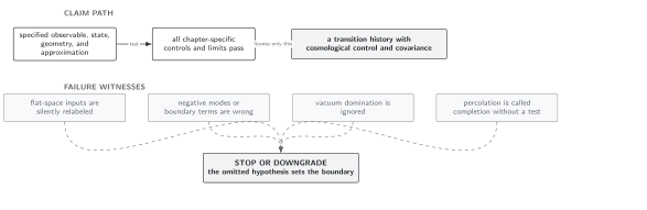
Failure conditions for global self-reproduction claims. The diagram is schematic and not to scale; a local decay rate remains meaningful even when a measure-independent global probability is unavailable.

These boundaries refine the chapter’s domain and failure conditions.

Exercise

In the constant-$H$, constant-$\Gamma$ benchmark, show that local survival tends to zero even when expected physical false volume grows.

Solution

At late times,

$$P_F(t)\sim \exp\!\left[-\frac{4\pi\Gamma}{3H^3}t\right],$$

which tends to zero for every $\Gamma>0$. Meanwhile,

$$a^3P_F\sim \exp\!\left[ \left(3H-\frac{4\pi\Gamma}{3H^3}\right)t \right].$$

The second expression grows when $\Gamma/H^4<9/(4\pi)$. One statement follows a given comoving region’s survival fraction; the other multiplies that fraction by exponentially growing physical volume.

References

• Freivogel, B. “Making Predictions in the Multiverse.” Classical and Quantum Gravity 28 (2011): 204007. DOI. Open PDF.
• Guth, A. H. “Eternal Inflation and Its Implications.” Journal of Physics A: Mathematical and Theoretical 40 (2007): 6811–6826. DOI. Open PDF.
• Vilenkin, A. “Birth of Inflationary Universes.” Physical Review D 27 (1983): 2848–2855. DOI.