Particle Creation in Time-Dependent Backgrounds

Time-dependent backgrounds create an in/out particle interpretation by mixing asymptotic positive and negative frequencies. The Bogoliubov coefficient $\beta_{\mathbf k}$ gives out occupation in the in-state when both asymptotic bases exist and are normalized. It does not by itself give a local energy density during the evolution, and a different out complex structure defines a different number observable.

Required background. Bogoliubov Transformations and Unitary Implementability supplies the representation criterion; Mode Bases, In/Out States, and Number Operators supplies asymptotic normalization.

Helpful background. In–Out versus In–In Expectation Values separates amplitudes from real-time expectation values; Adiabatic States, WKB Order, and Regularity supplies controlled approximate bases.

Bogoliubov evolution and occupation

For a homogeneous scalar background, each canonical mode can often be reduced to

$$v_{\mathbf k}'' +\omega_{\mathbf k}(\eta)^2v_{\mathbf k}=0, \qquad v_{\mathbf k}v_{\mathbf k}^{*'} -v_{\mathbf k}'v_{\mathbf k}^*=i.$$

Assume $\omega_{\mathbf k}\to\omega_{\mathbf k}^{\mathrm{in/out}}>0$ in stationary asymptotic regions. A normalized in-mode has future form

$$v_{\mathbf k}^{\mathrm{in}} \longrightarrow \frac{ \alpha_{\mathbf k}e^{-i\omega_{\mathbf k}^{\mathrm{out}}\eta} +\beta_{\mathbf k}e^{+i\omega_{\mathbf k}^{\mathrm{out}}\eta} }{ \sqrt{2\omega_{\mathbf k}^{\mathrm{out}}} }.$$

Wronskian conservation yields

$$\lvert\alpha_{\mathbf k}\rvert^2 -\lvert\beta_{\mathbf k}\rvert^2=1, \qquad n_{\mathbf k}^{\mathrm{out}} = \lvert\beta_{\mathbf k}\rvert^2$$

in the in-vacuum. The background supplies the energy. In a prescribed geometry or external field, backreaction is neglected only while the produced stress is small relative to the source that drives $\omega_{\mathbf k}$.

The late-time excess out energy for a diagonal free scalar state is

$$\Delta\rho_{\mathrm{out}} = \int\frac{\mathrm d^{d-1}k}{(2\pi)^{d-1}}\, \omega_{\mathbf k}^{\mathrm{out}} \lvert\beta_{\mathbf k}\rvert^2,$$

after the out-vacuum contribution is treated in the chosen renormalization scheme. During the quench, a local $\langle T_{\mu\nu}\rangle_{\mathrm{ren}}$ can also contain phase-sensitive interference terms and local vacuum-polarization terms. Number and local energy are therefore checked separately.

First application: an exactly smooth frequency quench

Take

$$\omega_{\mathbf k}^2(t) = \frac{ (\omega_{\mathbf k}^{\mathrm{in}})^2 +(\omega_{\mathbf k}^{\mathrm{out}})^2 }{2} +\frac{ (\omega_{\mathbf k}^{\mathrm{out}})^2 -(\omega_{\mathbf k}^{\mathrm{in}})^2 }{2} \tanh\frac{t}{\tau}.$$

Hypergeometric connection formulas give

$$\lvert\beta_{\mathbf k}\rvert^2 = \frac{ \sinh^2\!\left[ \frac{\pi\tau}{2} \left( \omega_{\mathbf k}^{\mathrm{out}} -\omega_{\mathbf k}^{\mathrm{in}} \right) \right] }{ \sinh(\pi\tau\omega_{\mathbf k}^{\mathrm{in}}) \sinh(\pi\tau\omega_{\mathbf k}^{\mathrm{out}}) }.$$

Das, Galante, and Myers give the exact modes, coefficients, and distinction between smooth-fast and instantaneous quenches Das, Galante, and Myers 2015, §2.

Two limits check the result. For $\tau\to0$ at fixed mode,

$$\lvert\beta_{\mathbf k}\rvert^2 \longrightarrow \frac{ \left( \omega_{\mathbf k}^{\mathrm{out}} -\omega_{\mathbf k}^{\mathrm{in}} \right)^2 }{ 4\omega_{\mathbf k}^{\mathrm{in}} \omega_{\mathbf k}^{\mathrm{out}} }.$$

For a slow quench with both asymptotic frequencies nonzero, production is exponentially suppressed. At large momentum the finite-$\tau$ result also falls exponentially, while an ideal instantaneous quench can have a much harder ultraviolet tail. The order of the $\tau\to0$ and cutoff limits is physical.

The number and energy densities are

$$n_{\mathrm{out}} = \int\frac{\mathrm d^{d-1}k}{(2\pi)^{d-1}} \lvert\beta_{\mathbf k}\rvert^2, \qquad \Delta\rho_{\mathrm{out}} = \int\frac{\mathrm d^{d-1}k}{(2\pi)^{d-1}} \omega_{\mathbf k}^{\mathrm{out}} \lvert\beta_{\mathbf k}\rvert^2.$$

Convergence of the first does not imply convergence of the second because the energy integral has an extra power of frequency.

Adversarial out-basis rotation

Keep the evolved state fixed and define a second out basis

$$\widetilde u_{\mathbf k}^{\mathrm{out}} = A_{\mathbf k}u_{\mathbf k}^{\mathrm{out}} +B_{\mathbf k}u_{-\mathbf k}^{\mathrm{out}*}, \qquad \lvert A_{\mathbf k}\rvert^2-\lvert B_{\mathbf k}\rvert^2=1.$$

The new production coefficient is a composition of the physical evolution with $(A,B)$, so $\lvert\widetilde\beta_{\mathbf k}\rvert^2$ generally differs. If the original out basis was selected by a future Killing generator and the rotated one is not, the latter number is still a mathematically valid basis occupation but has lost the asymptotic energy interpretation.

Local stress-energy, computed from the fixed two-point function with one fixed renormalization prescription, does not change under this relabeling. This is the decisive comparison: basis-dependent number changes, whereas the same local observable does not.

Construction and failure maps

The construction map places Bogoliubov evolution after asymptotic basis selection and before interpretation as number or energy.

In/out production is controlled by asymptotic normalization, canonical identities, ultraviolet convergence, and background energy balance; the map is schematic and not to scale.

The failure map identifies an unselected instantaneous or rotated basis as a failure witness, not as new invariant production.

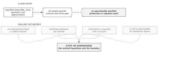
Only the number and energy associated with the declared asymptotic basis and controlled quench are licensed; the map is schematic and not to scale.

Use Domain and failure conditions. This page’s checks are Wronskian normalization, two asymptotic regimes, $\lvert\alpha\rvert^2-\lvert\beta\rvert^2=1$, wavepacket or density normalization, ultraviolet convergence, local-energy translation, and negligible backreaction.

Check your understanding

Can a quench have finite number density but divergent excess energy in an idealized sudden limit?

Solution

Yes. The energy integral weights each produced mode by $\omega_{\mathbf k}^{\mathrm{out}}$. A high-momentum tail can therefore be integrable for $\int n_{\mathbf k}$ but not for $\int\omega_{\mathbf k}n_{\mathbf k}$. A finite switching time or physical cutoff must remain when the instantaneous idealization exceeds its ultraviolet domain.

Adiabaticity, Stokes Phenomena, and Production Rates analyzes the complex-time origin of $\beta$. Chapter 2 owns representation selection, Chapter 6 collapse-induced production, and Chapter 14 cosmological deployment.

References

• N. D. Birrell and P. C. W. Davies, Quantum Fields in Curved Space, Cambridge University Press (1982), DOI, Chapter 3.
• Sumit R. Das, Damián A. Galante, and Robert C. Myers, “Smooth and Fast versus Instantaneous Quenches in Quantum Field Theory,” Journal of High Energy Physics 2015 (2015), article 73, DOI, arXiv:1505.05224.
• Leonard Parker, “Particle Creation in Expanding Universes,” Physical Review Letters 21 (1968), 562–564, DOI.