Black-Hole Thermodynamics at the QFT Interface

Semiclassical black-hole thermodynamics joins four logically distinct inputs: horizon kinematics fixes a temperature, quantum propagation fixes a greybody-filtered flux, a quantum state fixes local stress, and a renormalized gravitational action fixes geometric entropy. Their agreement in equilibrium is powerful, but none may be substituted for the others.

Required background. Hawking radiation from collapse supplies the late-time Bogoliubov calculation; black-hole states and greybody flux distinguishes Boulware, Hartle–Hawking, and Unruh states; and the renormalized stress tensor supplies the local energy source. Helpful background. Review the KMS condition, regulated subregion entropy, passivity, and Landauer processes.

Temperature, flux, and entropy are different observables

Let $\chi^a$ be the horizon-generating Killing field, normalized by the chosen asymptotic time, and $\kappa$ its surface gravity. A regular Euclidean section or the collapse calculation gives

$$T_H=\frac{\kappa}{2\pi},\qquad \langle N_{\omega\ell}\rangle_{\rm near\ horizon} =\frac{1}{e^{\omega/T_H}\mp1}.$$

The exponential relation between affine horizon frequency and asymptotic Killing frequency produces this Planck factor in the collapse calculation Hawking 1975, §§2–3, pp. 202–214.

At infinity the potential barrier multiplies this occupation by a transmission probability $\Gamma_{s\ell}(\omega)$, so in a four-dimensional asymptotically flat stationary geometry

$$\frac{dE}{dt\,d\omega} =\frac{1}{2\pi}\sum_{s,\ell}d_{s\ell} \frac{\omega\,\Gamma_{s\ell}(\omega)}{e^{\omega/T_H}-(-1)^{2s}}.$$

The thermal factor is obtained either from near-horizon KMS/Euclidean regularity or from the late-time collapse calculation after frequencies are related to the asymptotic Killing time; these are mutually consistent checks, not literally the same local observable. The resulting flux is not an entropy definition. The Unruh state has outgoing flux and is regular on the future horizon but is not a global equilibrium KMS state. The Hartle–Hawking state is the equilibrium comparison where it exists; the Boulware state is singular at the horizon. These distinctions follow from the state-dependent two-point function and stress tensor, not from $T_H$ alone Candelas 1980, §§II–IV, pp. 539–552.

For the renormalized Einstein–Hilbert action in the site’s Lorentzian convention, continuation of the full action gives the stationary geometric term

$$S_{\rm grav}=\frac{A_H}{4G_{\rm ren}}$$

for a smooth bifurcate Killing horizon. With angular momentum and charge, the stationary first law is

$$\delta M=T_H\,\delta S_{\rm grav}+\Omega_H\delta J+\Phi_H\delta Q.$$

It relates nearby stationary solutions. It does not assert monotonic entropy during unrestricted evaporation Wald 1993, pp. R3428–R3430.

First application: assemble one stationary case

For Schwarzschild mass $M$ in units $G=\hbar=c=k_B=1$,

$$r_H=2M,\qquad \kappa=\frac{1}{4M},\qquad T_H=\frac{1}{8\pi M},\qquad S_{\rm grav}=4\pi M^2.$$

Hence $dM=T_H\,dS_{\rm grav}$. To describe equilibrium, choose the Hartle–Hawking state and include both ingoing and outgoing thermal populations. To describe an isolated evaporating hole, choose the Unruh state, compute the greybody-filtered outgoing luminosity, and use the renormalized $\langle T_{ab}\rangle$ in a slow-backreaction equation. The negative mass change then belongs to a quasi-stationary approximation; it is not inferred from the equilibrium first law.

The chapter structure map locates this interface before the later entropy-renormalization and horizon-law steps. Inspect the separation between state-dependent QFT data and the geometric action term.

Stationary black-hole thermodynamics combines, but does not identify, horizon temperature, scattered flux, renormalized stress, and geometric entropy. Schematic; not to scale.

Domain and failure conditions

Use the chapter’s canonical domain table to compare this interface with generalized entropy, first laws, and the GSL. Here the decisive assumptions are a nonextremal Killing horizon, a normalization of $\chi^a$, a declared state, and perturbatively small backreaction.

Adversarial test. Apply $T=\kappa/(2\pi)$ and the stationary first law to a rapidly changing trapping horizon. There may be no Killing field, no unique normalization of $\kappa$, no Euclidean period, and no state regular enough to justify the stationary spectrum. At most one obtains a model-dependent adiabatic temperature when the evolution time is long compared with $\kappa^{-1}$; a general dynamical entropy law requires additional hypotheses.

The failure map highlights why “thermal spectrum,” “equilibrium state,” and “entropy increase” must be tested independently.

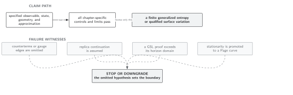
Stationary formulas fail in distinct ways when symmetry, scale separation, or state regularity is absent; none of those failures alone proves information loss. Schematic; not to scale.

Handoffs

Proceed to horizon entanglement entropy for the UV structure, semiclassical first laws for controlled variations, and the generalized second law for a genuine monotonicity statement.

References

• Candelas, P., “Vacuum Polarization in Schwarzschild Spacetime,” Physical Review D 21, 2185–2202 (1980), doi:10.1103/PhysRevD.21.2185.
• Hawking, S. W., “Particle Creation by Black Holes,” Communications in Mathematical Physics 43, 199–220 (1975), doi:10.1007/BF02345020.
• Wald, R. M., “Black Hole Entropy Is the Noether Charge,” Physical Review D 48, R3427–R3431 (1993), doi:10.1103/PhysRevD.48.R3427.