

Raychaudhuri Evolution, Null Focusing, and Renormalized Stress
Raychaudhuri’s equation converts local curvature along a null congruence into the evolution of its cross-sectional area. With quantum matter, the equation itself remains geometric; what changes is that the renormalized need not be pointwise nonnegative. A focusing conclusion therefore requires the initial expansion, shear, twist, affine normalization, stress prescription, and approximation order—not only the sign of one energy pulse.
Required background. Classical energy conditions and quantum violations supplies ; Levi–Civita connection and curvature supplies geodesic deviation; and globally hyperbolic spacetimes supplies the causal setting.
Helpful background. Null-smeared stress observables fixes the quantum source, while relativistic causality clarifies which later global inference requires more than local focusing.
Null expansion and its sign
Section titled “Null expansion and its sign”Let be tangent to an affinely parametrized null congruence in dimensions. The screen-space deformation decomposes into expansion , shear , and twist . With the site Riemann convention,
For generators orthogonal to a smooth null hypersurface, . With
null contraction removes both the trace and cosmological terms:
Thus NEC and nonzero shear make nonincreasing. If and NEC holds thereafter, dropping the other nonpositive terms gives
so diverges to no later than
This is a conjugate-point estimate, not by itself a singularity theorem. Geodesic incompleteness additionally needs global causal and genericity hypotheses; the separation between the local focusing lemma and the global causal argument is explicit in Wald 1984, Theorem 9.3.5 and § 9.5.
The structure map places Raychaudhuri between a renormalized null stress and any later causal consequence. Sampling or entropy conditions enter only when pointwise NEC is unavailable.

Null focusing with quantum matter. The map is schematic and not to scale; Raychaudhuri evolution is exact geometrically, while replacing curvature by a mean renormalized stress and deriving a global conclusion each require separate hypotheses.
A weak localized stress pulse
Section titled “A weak localized stress pulse”Take a twist-free, initially parallel congruence with negligible shear and
Assume , so the expansion generated by the pulse changes little over its own width and is perturbative. Integrating Raychaudhuri gives
A positive pulse produces negative expansion; a negative pulse defocuses at this order. This is an initial-value result for the mean geometry. It does not say that an isolated negative pulse is an allowed complete quantum history; a QEI or ANEC statement may constrain the state and accompanying stress elsewhere.
After a positive pulse, suppose and shear remains zero. The exact vacuum evolution is
For , a caustic occurs after affine interval . If shear is generated by the pulse, moves the caustic earlier. Omitting shear can therefore overestimate, not underestimate, the available affine distance.
Affine-normalization adversarial test
Section titled “Affine-normalization adversarial test”Under with ,
The jump law becomes , and the affine distance to the caustic scales by . The spacetime event is unchanged. Quoting or a focusing length without the normalization of is therefore meaningless.
A second adversarial run sets the initial shear to a localized nonzero profile but solves the shear-free equation. Comparing with the full equation exposes a missed negative contribution. The correction is physical and cannot be repaired by rescaling .
The failure map highlights these two errors: hidden affine normalization changes numerical bounds, whereas omitted shear changes the actual congruence.
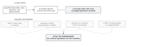
Failure tests for a Raychaudhuri calculation. The diagram is schematic and not to scale; affine rescaling must transform tangent, expansion, stress projection, integration measure, and endpoints together.
Domain and failure conditions
Section titled “Domain and failure conditions”See the chapter domain and failure-conditions table. The pulse calculation assumes an affine, twist-free congruence, a fixed renormalized mean stress, negligible shear at the retained order, and weak backreaction during the pulse. It fails for nonaffine generators unless the nonaffinity term is restored, near caustics where linearization fails, or when fluctuation effects invalidate a mean-stress geometry.
Exercise
Section titled “Exercise”Integrate from and locate the caustic.
Solution
Separation gives , hence
The denominator vanishes at .
References
Section titled “References”- Wald, R. M. General Relativity. University of Chicago Press, 1984. Publisher.
Original QFT.org content:CC BY 4.0, unless an item supplies different terms. Third-party material retains its own terms.