

Locality, Contact Ambiguities, and Field-Redefinition Equivalence
Bulk locality constrains the allowed singularities and large-energy growth of cosmological coefficients, but it does not make individual contact coefficients invariant. Integration by parts, equations of motion, local field redefinitions, and finite boundary counterterms move analytic data while preserving properly translated observables and nonlocal propagation.
Required background. Contact and exchange seeds and factorization singularities identify local and nonlocal pieces. Local field redefinitions and the equivalence theorem supplies the EFT quotient, while renormalized contact products supplies operator-contact freedom.
Helpful background. Large-N contact ambiguities provide a related boundary example, and causality and analytic growth domains clarify what extra input locality tests require.
Local representatives and invariant content
Section titled “Local representatives and invariant content”Consider a scalar with free equation
The identity
shows why “use the equations of motion” is incomplete on a finite cosmological time interval. Replacing by converts the bulk derivative vertex into a nonderivative contact, but the late-boundary term remains.
More generally, under a perturbatively invertible local change
the free action changes as
The equation-of-motion operator is redundant only together with the boundary functional, Jacobian or counterterms at the working order, and the transformation of external observables. The flat-space equivalence theorem makes the analogous statement for local invertible transformations and asymptotic amplitudes (Kamefuchi, O’Raifeartaigh, and Salam 1961, §§ 2–3). Cosmology has a finite late boundary rather than out states, so raw boundary-field correlators are expected to change.
Cubic-action application
Section titled “Cubic-action application”Compare
with the representative obtained from the identity above,
up to an operator proportional to . Direct wavefunction time integrals distribute analytic terms differently between the bulk and late boundary. At order , eliminating the redundant cubic also generates quartic contacts. Once those terms and the external-field map are included:
- the physical internal mass and nonanalytic exchange branch are unchanged;
- partial-energy residues agree in translated observables;
- local wavefunction contacts and raw components can differ.
Maldacena performs precisely this kind of separation between equation-of-motion cubic terms and a nonlinear field redefinition in the inflationary bispectrum (Maldacena 2003, Eqs. (3.9)–(3.12) and (4.3)–(4.5)).
Analytic locality tests
Section titled “Analytic locality tests”Within an EFT truncated at derivative order , a candidate coefficient should pass:
- factorization: every physical nonlocal channel has the residue or discontinuity dictated by lower-point data;
- spurious-singularity cancellation: denominators not associated with total or allowed partial energies cancel in the sum;
- large-energy growth: after the declared subtractions, scaling does not exceed that implied by ;
- soft behavior: gauge and adiabatic Ward identities hold, including contact sources;
- contact-basis closure: the remaining analytic freedom is spanned by local operators through order .
Passing these tests establishes compatibility with the stated local EFT class. It does not prove microscopic locality at arbitrarily high energy. A sufficiently complicated nonlocal kernel can mimic finitely many terms of a derivative expansion.
Boundary counterterms deserve separate notation. A polynomial in external momenta can be local on the late slice while not corresponding to a bulk interaction. Such terms may change the wavefunction phase without changing an equal-time probability, or change composite-operator contacts without changing separated-point data.
Equivalent-actions adversarial test
Section titled “Equivalent-actions adversarial test”Generate a family of representatives by:
For each, compute the cubic coefficient, the induced quartic contact, and a four-point exchange coefficient. Translate the external operator and compare:
All must agree. The contact decomposition need not. Reject any proposed “locality discriminator” that assigns different physical content solely because the representatives have different analytic polynomials.
The structure map shows the quotient between raw coefficients and physical nonlocal data. Inspect how boundary and field-redefinition branches rejoin before reconstruction.

Locality tests after quotienting contact and field-basis freedom. The diagram is schematic and not to scale; the derivative order and boundary conditions define the tested EFT class.
The failure map distinguishes raw contact differences from physical failures. Inspect the stops for dropping an endpoint term, omitting an induced quartic, or comparing untransformed external fields.
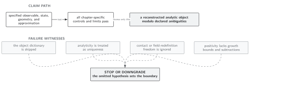
Failure conditions for locality and field-redefinition tests. The diagram is schematic and not to scale; local contact coefficients are representatives, whereas nonlocal channel data are the robust comparison.
These rules refine the chapter’s domain and failure conditions. They determine the polynomial freedom retained by dispersion relations and reconstruction.
Exercise
Section titled “Exercise”Derive the integration-by-parts identity used above.
Solution
Apply the product rule:
Integrating and using the divergence theorem gives
The boundary contribution vanishes only under boundary conditions that make it zero.
References
Section titled “References”- Kamefuchi, S., L. O’Raifeartaigh, and A. Salam. “Change of Variables and Equivalence Theorems in Quantum Field Theories.” Nuclear Physics 28 (1961): 529–549. DOI.
- Maldacena, J. “Non-Gaussian Features of Primordial Fluctuations in Single Field Inflationary Models.” Journal of High Energy Physics 2003, no. 05 (2003): 013. DOI. Open PDF.
Original QFT.org content:CC BY 4.0, unless an item supplies different terms. Third-party material retains its own terms.