Switching, Smearing, Finite-Time Response, and Transients

Switching and spatial smearing are physical parts of a localized measurement, not disposable technicalities. They determine spectral bandwidth, inject control energy, regulate the pullback of singular correlations, and set the transient error in any proposed rate. Smooth finite protocols give a well-defined probability; stationary rates require an additional long-time limit with its order of limits declared.

Required background. Detector Response Along Curved and Accelerated Worldlines supplies the response function; Switching, Smearing, and Detector Regularization supplies the general regulator framework.

Helpful background. Detector and instrument validation supplies control comparisons; Products, Scaling Degree, and Extensions of Singular Distributions explains why singular limits can fail.

Finite response and spectral resolution

For a stationary pulled-back two-point function with spectral density $\dot{\mathcal F}(\omega)$, smooth switching gives schematically

$$\mathcal F_\chi(\Omega) = \frac{1}{2\pi} \int_{-\infty}^{\infty}\mathrm d\nu\, \lvert\widehat\chi(\nu)\rvert^2 \dot{\mathcal F}(\Omega+\nu),$$

with the precise Fourier signs fixed by the convention for $\widehat\chi$. Switching therefore convolves the stationary spectrum with the apparatus bandwidth.

For a scaled family $\chi_T(\tau)=\chi(\tau/T)$,

$$\widehat\chi_T(\nu)=T\widehat\chi(T\nu).$$

Under suitable integrability and stationarity assumptions,

$$\mathcal F_{\chi_T}(\Omega) = T\,C_\chi\,\dot{\mathcal F}(\Omega)+O(1), \qquad C_\chi=\int\mathrm d\tau\,\lvert\chi(\tau)\rvert^2.$$

The $O(1)$ term is a switching transient. Dividing by $TC_\chi$ and taking $T\to\infty$ recovers the stationary rate. At finite $T$, it must not be silently discarded.

A spatial profile $F(\boldsymbol\xi)$ in Fermi–Walker coordinates replaces the point field by

$$\Phi_F(\tau) = \int\mathrm d^3\xi\, F(\boldsymbol\xi)\Phi(x(\tau,\boldsymbol\xi)).$$

Its Fourier transform suppresses wavelengths shorter than the detector size. The pointlike limit and sharp-switching limit probe different ultraviolet directions and need not commute. Schlicht showed why a rigid spatial profile resolves otherwise problematic accelerated-detector regularization Schlicht 2004, §§2–4.

First application: Gaussian and compact switching

Compare

$$\chi_G(\tau) = e^{-\tau^2/(2T^2)}$$

with a smooth compactly supported bump $\chi_C(\tau/T)$ normalized to the same $C_\chi$. The Gaussian has rapidly decaying frequency tails but never vanishes exactly in time. The compact bump is exactly localized; its spectral tail depends on its differentiability and edge shape.

For a stationary detector, compute

$$\delta\mathcal F_\chi(\Omega) = \mathcal F_\chi(\Omega) -TC_\chi\dot{\mathcal F}(\Omega).$$

Repeating the calculation for increasing $T$ separates the common linear stationary term from profile-dependent transients. Agreement of the extracted rate under both families, with $\delta\mathcal F/(TC_\chi)\to0$, is a regulator control. A single switching profile at one duration is not.

Smooth switching also makes the response well defined for a detector in an arbitrary Hadamard state on a four-dimensional curved spacetime Louko and Satz 2008, §§2–4. This uses the ultraviolet form of the state; a non-Hadamard two-point function can defeat the same protocol.

Adversarial order of limits

Let the spatial width $\epsilon\to0$ and switching rise time $\delta\to0$. If one first replaces $\chi$ by a step function and then removes the point-splitting or profile regulator, contact singularities can produce a divergent probability or a regulator-dependent constant. Reversing the limits can give a different answer.

The repair is not to rename the divergent term “particle creation.” Keep a smooth finite protocol, extract a transition rate through a proved long-time or controlled sharp-switching limit, and report which transient or counterterm has been removed. Louko and Satz show that a suitable zero-size detector rate can be profile independent under explicit hypotheses Louko and Satz 2006, §§3–4; this does not license every simultaneous sharp limit.

Construction and failure maps

The structure map places switching and smearing before the response calculation because they define the operation being performed.

Finite duration and detector size set the response bandwidth and transient error; the construction map is schematic and not to scale.

The validity map identifies the page’s failure witness directly: omitted switching transients can imitate a state population or spoil detailed balance.

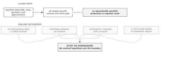
A stationary rate is licensed only after protocol families, ultraviolet limits, and transient scaling have been controlled; the map is schematic and not to scale.

The detector row of Domain and failure conditions lists the shared inputs. Here the decisive quantities are $T$, rise time, profile width, gap, perturbative parameter, Fourier tail, regulator, and the order in which long-time, sharp, and pointlike limits are taken.

Check your understanding

Why can two switchings with the same duration give different finite excitation probabilities but the same asymptotic rate?

Solution

Their Fourier windows and edge transients differ, producing different $O(1)$ contributions. If both scaled families concentrate at zero frequency as $T\to\infty$, the leading $TC_\chi\dot{\mathcal F}(\Omega)$ term is the same after normalization. Equality of the rate is an asymptotic result, not equality of finite protocols.

Unruh Effect and Uniformly Accelerated Detectors applies the long-time test. General detector regularization remains in Volume XIII, and distribution-extension theorems remain in Volume I.

References

• Jorma Louko and Alejandro Satz, “How Often Does the Unruh–DeWitt Detector Click? Regularisation by a Spatial Profile,” Classical and Quantum Gravity 23 (2006), 6321–6344, DOI, arXiv:gr-qc/0606067.
• Jorma Louko and Alejandro Satz, “Transition Rate of the Unruh–DeWitt Detector in Curved Spacetime,” Classical and Quantum Gravity 25 (2008), 055012, DOI, arXiv:0710.5671.
• Sebastian Schlicht, “Considerations on the Unruh Effect: Causality and Regularization,” Classical and Quantum Gravity 21 (2004), 4647–4660, DOI, arXiv:gr-qc/0306022.