Relativistic Protocols, Clocks, Encoding, and Channel Tomography

A reproducible relativistic protocol records clocks, synchronization, local frames, wavepacket bases, calibration data, and the map used to transform them. Channel tomography estimates parameters relative to those choices. A change of clock or basis transforms gain and covariance in a calculable way; applying it to the data but not the calibration can mimic channel drift.

Required background. Accelerated Detector Communication Channels supplies proper-time response. Entanglement Distribution and State Transfer Through Curved Fields fixes the decoded task. Relativistic Communication Protocols: Assumptions and Status supplies the protocol categories.

Helpful background. Wavepackets, Modes, Frames, and Localization fixes the mode basis. Detector, Channel, and Local-Parameter Tomography supplies statistical reconstruction. Entanglement Witnesses and Local Tomography Limits limits accessible certification. Quantum Energy Teleportation provides a protocol in which timing and local energy accounting are especially consequential.

A protocol record in spacetime

For each run, specify:

• sender and receiver worldtubes, tetrads, and proper-time functions $\tau_A(t),\tau_B(t)$;
• the synchronization event or exchanged timing signals and their uncertainty;
• normalized input and output wavepacket functions, including polarization and bandwidth;
• preparation maps, localized interaction densities, switching supports, and detector reset;
• receiver POVMs, digitization, postselection, and accessible algebra;
• the geometry and field state model used to predict propagation;
• code energy, sample size, drift model, and confidence construction.

A coordinate timestamp does not replace a clock reading. For a static metric, $d\tau_\nu=N_\nu dt$; for an accelerated laboratory, $\tau_\nu(t)$ is generally nonlinear. Switching functions written in $t$ and $\tau$ describe the same intervention only when the Jacobian and support transformation are included.

Gaussian tomography

For a weak linear channel, estimate

$$d_B=X d_A+d_0, \qquad V_B=X V_A X^T+Y.$$

Prepare at least a spanning set of input displacements $d_A^{(k)}$ and measure receiver first moments to estimate $X,d_0$. Use calibrated covariance inputs to estimate $Y$. A physical reconstruction must satisfy

$$Y+\frac{i}{2}(\Omega_B-X\Omega_A X^T)\ge0.$$

If an unconstrained least-squares estimate violates this inequality within uncertainty, project to a physical model only with the projection rule reported; otherwise the “channel” may be a statistical artifact. Quantum process tomography was demonstrated optically with coherent-state probes by Lobino et al. 2008, pp. 563–566, but a curved deployment additionally needs the spacetime support and frame transformations above.

To test signaling support, include sender-off runs and at least one causally disjoint timing fixture. The estimated sender-dependent block $X_{BA}$ should vanish in the latter within uncertainty. State noise can remain in $Y$.

Two clock and quadrature conventions

Consider static laboratories. Let $\Omega_\nu$ be the local proper-time oscillator frequency and $\bar\Omega_\nu=N_\nu\Omega_\nu$ its Killing-time frequency. Define proper-time normalized quadratures

$$R_\nu^{(\tau)} =\begin{pmatrix}\sqrt{\Omega_\nu}q_\nu\\p_\nu/\sqrt{\Omega_\nu}\end{pmatrix}$$

and coordinate-time normalized quadratures

$$R_\nu^{(t)} =D_\nu R_\nu^{(\tau)}, \qquad D_\nu= \begin{pmatrix}\sqrt{N_\nu}&0\\0&1/\sqrt{N_\nu}\end{pmatrix}.$$

Because $D_\nu$ is symplectic, this is a convention change, not a physical channel. If tomography in the proper-time convention gives $(X^{(\tau)},Y^{(\tau)},d_0^{(\tau)})$, the same data expressed in the coordinate-time convention give

$$X^{(t)}=D_BX^{(\tau)}D_A^{-1}, \qquad Y^{(t)}=D_BY^{(\tau)}D_B^T, \qquad d_0^{(t)}=D_Bd_0^{(\tau)}.$$

For an isotropic proper-time gain $X^{(\tau)}=gI$, the two coordinate-time quadrature gains are

$$g_q=g\sqrt{\frac{N_B}{N_A}}, \qquad g_p=g\sqrt{\frac{N_A}{N_B}}.$$

Reporting one of these as a physical amplification while retaining $Y^{(\tau)}$ would be inconsistent. The complete transformation preserves the CP inequality and all coordinate-independent predictions after preparations and measurements are transformed too.

Tomographic application and uncertainty

Estimate a weak curved-field link twice:

1. label switching, wavepacket phases, and quadratures by each laboratory’s proper time;
2. relabel the same raw events by the stationary coordinate time and apply $D_A,D_B$.

Fit $X,Y$ independently in both descriptions. The transformed confidence region from the first fit should contain the second. A convenient residual is

$$\delta_X= \left\lVert X^{(t)}_{\rm fit}-D_BX^{(\tau)}_{\rm fit}D_A^{-1} \right\rVert,$$

with a corresponding covariance residual for $Y$. Bootstrap or likelihood sampling must transform calibration nuisance parameters jointly, including lapse uncertainty and mode-center uncertainty.

The result is a model calculation or instrument estimate, depending on whether the data are simulated or measured. It establishes the channel only over the calibrated code subspace and energy range. It does not establish a capacity without a coding experiment or theorem, and it does not validate a curved-background model if competing propagation models fit equally well.

Synchronization and mode-basis adversary

After calibration, shift the receiver clock origin by $\delta\tau_B$ without updating the decoded mode. A frequency component acquires phase $e^{-i\Omega_B\delta\tau_B}$, so a stationary channel appears to rotate. Likewise replace output mode $v$ by $v'$ while continuing to divide by the old efficiency. Apparent changes in gain or noise then arise from a convention mismatch.

Reanalyze with the phase rotation and basis overlap included. If the drift disappears, no physical change was detected. If it persists and exceeds the propagated calibration uncertainty in both conventions, a physical or instrumental change remains possible. Distinguishing those requires environmental controls, repeated reference runs, and a specified alternative model.

Domain, limits, and maps

The canonical table is Domain and failure conditions. Finite probe sets certify only a model class; Gaussian tomography cannot exclude small non-Gaussian terms without additional tests. Clock synchronization is itself a physical protocol with delay and uncertainty. In nonstationary spacetime there may be no global $t$ or conserved frequency, so transformations must be local and run dependent.

The structure map makes calibration part of both endpoints. Inspect the frame-transformation checkpoint before interpreting a fitted gain as curvature or acceleration.

Gain and noise are meaningful only relative to transformed sender and receiver frames, calibrated instruments, and a declared code subspace. Schematic; not to scale.

The failure map stops an apparent drift when clock or wavepacket conventions have changed asymmetrically. Transforming both the fit and calibration is the countertest.

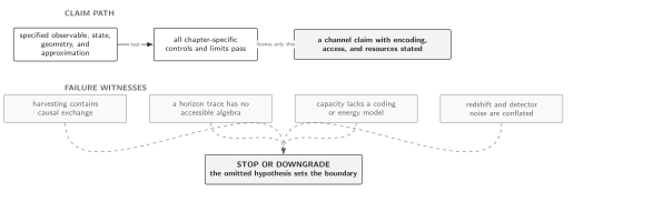
Only residual change after joint clock, frame, basis, and uncertainty transformation can be assigned to physics or apparatus. Schematic; not to scale.

Handoffs

Evidence, Analogue Systems, and Astrophysical Claim Limits classifies what a measured platform can establish. Detector, Channel, and Local-Parameter Tomography owns general estimators and confidence methods. A bounded calculation can check the same quantities.

References

• Lobino, Mirko, Dmitry Korystov, Connor Kupchak, Eden Figueroa, Barry C. Sanders, and A. I. Lvovsky. “Complete Characterization of Quantum-Optical Processes.” Science 322 (2008): 563–566. DOI. Open PDF.
• Šafránek, Dominik. “Estimation of Gaussian Quantum States.” Journal of Physics A: Mathematical and Theoretical 52 (2019): 035304. DOI. Open PDF.