Initial Density Matrices and Boundary EFT

A cosmological initial condition is most generally a positive normalized state functional on the observables of an initial Cauchy surface, not a mode-by-mode slogan about positive frequency. In the regulated canonical description used here—one may begin in a finite comoving box before taking the continuum limit—the state is represented by a density operator. On a closed time path, its field-basis kernel joins the forward and backward fields at the initial boundary. This page makes the construction explicit for a Gaussian scalar state, derives the state-dependent propagator, and separates positivity and normalization from the additional assumptions of a boundary effective field theory.

Required background. Vacuum choice and initial states supplies normalized reference modes; initial density matrices on real-time contours supplies the two branches; and controlled EFT expansions supplies power counting. Helpful background. Curvature counterterms distinguish bulk from surface renormalization.

Density matrices are initial-boundary data

Let the initial surface be $\Sigma_0$ at conformal time $\eta_0$. In the field basis,

$$\langle\varphi_+|\rho_0|\varphi_-\rangle =\mathcal N\exp\!\left(iS_0[\varphi_+,\varphi_-]\right).$$

The labels $+$ and $-$ denote fields evolved respectively by $U$ and $U^\dagger$. Hermiticity requires

$$S_0[\varphi_+,\varphi_-]^* =-S_0[\varphi_-,\varphi_+],$$

while positivity means $\langle\psi|\rho_0|\psi\rangle\geq0$ for every state $|\psi\rangle$. The constant $\mathcal N$ is fixed by $\operatorname{Tr}\rho_0=1$. Equivalently, after the final fields are identified and integrated over, the normalized Schwinger–Keldysh functional obeys $Z[J,J]=1$. The diagonal kernel $\rho_0[\varphi,\varphi]$ is generally not equal to one and does not vanish; its integral is the trace.

The initial insertion, the two bulk histories, and their final trace have distinct jobs. Agarwal, Holman, Tolley, and Lin develop this density-matrix path integral and its Gaussian Green functions in Agarwal et al. 2013, §2 and Appendix A.

The diagram shows where each ingredient lives. In particular, surface counterterms renormalize short-distance structure attached to $\Sigma_0$; they are not extra bulk interactions.

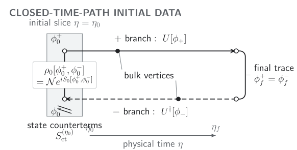
The density matrix couples the $+$ and $-$ fields only at the initial surface; unitary bulk evolution carries them to a common final field that is integrated over in the trace. Boundary counterterms remain localized at $\eta_0$. Schematic; not to scale.

The machine-readable figure description records the branches, orientations, labels, and scope without relying on the image.

One Gaussian mode in exact form

Before treating a field, consider one real canonical degree of freedom with $[q,p]=i$, zero mean, and covariance

$$\Gamma= \begin{pmatrix} Q&S\\ S&P \end{pmatrix}, \qquad Q=\langle q^2\rangle, \quad P=\langle p^2\rangle, \quad S=\frac12\langle qp+pq\rangle.$$

Set $q_r=(q_++q_-)/2$, $q_a=q_+-q_-$, and $D=QP-S^2$. The normalized Gaussian density kernel is

$$\langle q_+|\rho|q_-\rangle =\frac{1}{\sqrt{2\pi Q}} \exp\!\left[ -\frac{q_r^2}{2Q} -\frac{Dq_a^2}{2Q} +i\frac{S}{Q}q_rq_a \right].$$

The uncertainty condition $\Gamma+i\Omega/2\geq0$ reduces, for one mode, to

$$Q>0, \qquad D=QP-S^2\geq\frac14.$$

The equality $D=1/4$ describes a pure Gaussian state; $D>1/4$ describes a mixed one. Thus purity and positivity are visible directly in the boundary kernel, without choosing a particle interpretation.

For a homogeneous real field, choose normalized reference modes $v_k$ and reference operators $a_{\boldsymbol k}$. Write

$$\langle a_{\boldsymbol k}^\dagger a_{\boldsymbol q}\rangle =(2\pi)^3\delta^3(\boldsymbol k-\boldsymbol q)N_k, \qquad \langle a_{\boldsymbol k}a_{\boldsymbol q}\rangle =(2\pi)^3\delta^3(\boldsymbol k+\boldsymbol q)C_k.$$

For the reference oscillator of frequency $\omega_k$,

$$Q_k=\frac{N_k+\frac12+\operatorname{Re}C_k}{\omega_k}, \qquad P_k=\omega_k\!\left(N_k+\frac12-\operatorname{Re}C_k\right), \qquad S_k=\operatorname{Im}C_k.$$

Consequently,

$$N_k\geq0, \qquad |C_k|^2\leq N_k(N_k+1).$$

These are necessary and sufficient positivity conditions for each independent Gaussian mode. A pure squeezed state saturates the second inequality; a thermal or otherwise mixed state does not. This is why replacing a general density matrix by one Bogoliubov-transformed mode loses part of the problem.

The modified propagator

Expand the field mode as

$$\varphi_{\boldsymbol k}(\eta) =v_k(\eta)a_{\boldsymbol k} +v_k^*(\eta)a_{-\boldsymbol k}^\dagger.$$

Its statistical two-point function is

$$\begin{aligned} F_k(\eta,\eta') ={}&\frac12\left\langle \{\varphi_{\boldsymbol k}(\eta), \varphi_{-\boldsymbol k}(\eta')\}\right\rangle\\ ={}&\left(N_k+\frac12\right) \left[v_k(\eta)v_k^*(\eta')+v_k^*(\eta)v_k(\eta')\right]\\ &+C_kv_k(\eta)v_k(\eta') +C_k^*v_k^*(\eta)v_k^*(\eta'). \end{aligned}$$

By contrast, the commutator is

$$\Delta_k(\eta,\eta') =\left\langle [\varphi_{\boldsymbol k}(\eta), \varphi_{-\boldsymbol k}(\eta')] \right\rangle =v_k(\eta)v_k^*(\eta')-v_k^*(\eta)v_k(\eta').$$

All dependence on $N_k$ and $C_k$ cancels from $\Delta_k$. The two Wightman functions are $G_k^>=F_k+\Delta_k/2$ and $G_k^<=F_k-\Delta_k/2$; contour ordering then builds the four $G_k^{ab}$. Relative to the reference vacuum, the exact Gaussian correction is therefore

$$\delta F_k =N_k\left[v_kv_k^*+v_k^*v_k\right] +C_kv_kv_k+C_k^*v_k^*v_k^*, \qquad \delta\Delta_k=0,$$

where the time arguments follow the preceding displayed equation. This is the promised modified propagator: in this free linear benchmark, initial occupation and pair coherence change statistical correlations, while the free equation, Wronskian jump, and causal support remain fixed. A free calculation that changes the commutator when only $\rho_0$ was changed has accidentally changed the dynamics or the canonical normalization. Interacting retarded correlators can themselves be state dependent and require a separate analysis.

When a boundary EFT is justified

A density matrix and a boundary EFT are related but not identical notions. Any admissible state supplies initial data. A boundary EFT is an additional low-energy ansatz: over a specified physical-momentum window $p=k/a_0<\Lambda$, its short-distance dependence is organized in local operators on $\Sigma_0$, for example

$$S_{0,\mathrm{EFT}} =\int_{\Sigma_0}d^3x\sqrt h \left[ \frac{\kappa}{2}\phi^2 +\frac{c_1}{2\Lambda}h^{ij}D_i\phi D_j\phi +\cdots \right],$$

together with the doubled and mixed kernels required on the closed time path. The coefficients depend on a renormalization prescription; observables do not, up to the first omitted power of $p/\Lambda$.

Loops then separate into ordinary bulk divergences and, for the specified effective initial structure, divergences supported at $\eta_0$. The latter are canceled by local surface operators. Collins and Holman derive this separation and boundary running in Collins and Holman 2005, §§II–IV; for the stress tensor, the needed initial-surface geometric counterterms are exhibited in Collins and Holman 2006, §§II–IV.

This statement should not be reversed: an ordinary Hadamard state does not, merely by being a state, demand state-dependent counterterms. The boundary-EFT counterterms renormalize a chosen finite-time effective parameterization of ultraviolet deviations. The physical expansion parameter is $p/\Lambda=k/(a_0\Lambda)$, not comoving $k/\Lambda$.

Checks and failure conditions

Before using a Gaussian initial state, verify all of the following:

• Density operator: $\operatorname{Tr}\rho_0=1$, Hermiticity, and $|C_k|^2\leq N_k(N_k+1)$.
• Canonical evolution: the reference modes satisfy the Wronskian, and the state changes $F_k$ but not $\Delta_k$.
• Ultraviolet domain: the state returns smoothly enough to an admissible reference state above its preparation scale, or the calculation states the finite cutoff and its completion.
• EFT control: every retained mode obeys $k/(a_0\Lambda)\ll1$, and the first omitted boundary operator is smaller than the claimed effect.
• Renormalization: bulk and initial-surface counterterms are distinguished, and residual dependence on the subtraction scale is of omitted order.

An instructive failure is to hold an unsuppressed excitation fixed while sending the comoving cutoff to infinity at fixed $a_0$. The excitation energy and surface divergences then grow without an EFT hierarchy. A second failure is to choose $|C_k|^2>N_k(N_k+1)$: the resulting covariance violates the uncertainty principle, so no positive density operator exists.

Common pitfalls

Confusing equal histories with a trivial density kernel. The identity $Z[J,J]=1$ follows only after the two histories are joined and traced. It does not imply $\rho_0[\varphi,\varphi]=1$ pointwise.

Using the same symbols for two different parameterizations. Boundary-action kernels and Bogoliubov coefficients are different objects. Here $N_k,C_k$ describe covariance data; the next pages reserve $\alpha_k,\beta_k$ for mode mixing.

Calling every finite-time state a boundary EFT. Local power counting, a declared cutoff, and a renormalization prescription are extra hypotheses. Without them, the density matrix may still define a state, but it does not define a controlled EFT extrapolation.

Exercises

For the one-mode kernel above, verify normalization and derive the positivity bound.

Solution

On the diagonal, $q_a=0$ and $q_r=q$, so

$$\operatorname{Tr}\rho =\int dq\,\frac{e^{-q^2/(2Q)}}{\sqrt{2\pi Q}}=1.$$

The covariance of one canonical pair is physical exactly when $\Gamma+i\Omega/2\geq0$, with $\Omega_{qp}=1$. Its determinant condition is $QP-S^2\geq1/4$. Substituting the $N,C$ parameterization gives

$$QP-S^2 =\left(N+\frac12\right)^2-|C|^2\geq\frac14,$$

or $|C|^2\leq N(N+1)$. Positivity of $Q$ also implies $N\geq0$ for the occupation-number covariance. Equality gives a pure Gaussian; strict inequality gives a mixed state.

Starting from the mode expansion, derive $F_k$ and $\Delta_k$ and show explicitly which one carries the state data.

Solution

Use $\langle a^\dagger a\rangle=N$, $\langle aa^\dagger\rangle=N+1$, $\langle aa\rangle=C$, and $\langle a^\dagger a^\dagger\rangle=C^*$. Adding the two operator orderings gives

$$F_k=\left(N_k+\frac12\right)(v_kv_k^*+v_k^*v_k) +C_kv_kv_k+C_k^*v_k^*v_k^*,$$

with the two time arguments kept in their original order. Subtracting the orderings cancels $N_k$ and $C_k$ and leaves $\Delta_k=v_kv_k^*-v_k^*v_k$. Thus the density matrix changes the symmetric fluctuations but not the canonical commutator. At equal times,

$$F_k(\eta,\eta) =(2N_k+1)|v_k(\eta)|^2 +2\operatorname{Re}\!\left[C_kv_k(\eta)^2\right],$$

which displays separately the occupation and pair-coherence contributions.

References

• Agarwal, N., R. Holman, A. J. Tolley, and J. Lin, “Effective Field Theory and Non-Gaussianity from General Inflationary States,” Journal of High Energy Physics 2013, 085 (2013), doi:10.1007/JHEP05(2013)085, Open PDF.
• Collins, H., and R. Holman, “Renormalization of Initial Conditions and the Trans-Planckian Problem of Inflation,” Physical Review D 71, 085009 (2005), doi:10.1103/PhysRevD.71.085009.
• Collins, H., and R. Holman, “The Renormalization of the Energy-Momentum Tensor for an Effective Initial State,” Physical Review D 74, 045009 (2006), doi:10.1103/PhysRevD.74.045009.