Applying EFT Power Counting to Gravity

Gravity EFT is ordered by the size of a declared observable, not by operator dimension alone. Canonical normalization converts every graviton interaction into powers of $1/M_{\mathrm{Pl}}$; derivatives, background curvature, loop factors, active species, Wilson coefficients, and duration then determine which terms compete.

Required background. Effective Field Theory of Gravity: Architecture and Power Counting fixes the gravitational EFT setup; Power Counting and Predictive Order fixes operator ordering; and Effective Field Theory as a Controlled Expansion fixes remainder claims.

Helpful background. Loops, Counterterms, and Closure of an EFT Expansion supplies loop closure, while Modes, Virtualities, and EFT Scale Separation separates scales.

Canonical graviton counting

Use the site action

$$S_{\mathrm{EH}} =-\frac{M_{\mathrm{Pl}}^2}{2}\int\mathrm d^4x\sqrt{-g}\,(R-2\Lambda), \qquad g_{\mu\nu}=\bar g_{\mu\nu}+\frac{2h_{\mu\nu}}{M_{\mathrm{Pl}}}.$$

An Einstein–Hilbert vertex with $n$ canonically normalized gravitons has schematic size

$$\mathcal V_n^{\mathrm{EH}} \sim \frac{p^2}{M_{\mathrm{Pl}}^{\,n-2}}.$$

For a connected graph with $L$ loops, each graviton or ghost loop adds $p^2/(16\pi^2M_{\mathrm{Pl}}^2)$ after topological identities are used. A matter loop has the same gravitational vertices but carries its spin and species multiplicity. An insertion $C_d\mathcal O_d$ with $d$ derivatives is measured relative to an EH vertex by

$$\epsilon_d(p) \sim \frac{C_dp^{d-2}}{M_{\mathrm{Pl}}^2}.$$

For $C_d\sim M_{\mathrm{Pl}}^2/\Lambda^{d-2}$ this becomes $(p/\Lambda)^{d-2}$; that coefficient estimate is an assumption, not an EFT theorem. On a background, derivatives and curvature count separately. If $\mathcal R$ is the largest independent curvature scale sampled in the observable’s physical tetrad, then

$$p^2\longleftrightarrow \max\!\left(p^2,\mathcal R\right)$$

only as an order estimate. Tensor contractions and symmetries can remove the apparent leading term.

The structure map begins here because every later basis, loop, and matching decision consumes this count.

Canonical normalization turns gravitational vertices into Planck-suppressed interactions; derivative, curvature, loop, and species factors then order a particular amplitude or background response. The map is schematic and not to scale.

First application: one graviton–matter process

Consider a dimensionless low-energy $2\to2$ amplitude at characteristic invariant $E^2\ll M_{\mathrm{Pl}}^2$ and weak background curvature. Its leading gravitational scaling is

$$\mathcal A_{\mathrm{tree}}\sim\frac{E^2}{M_{\mathrm{Pl}}^2}.$$

A one-loop correction with $N_{\mathrm{eff}}(E)$ active matter species and declared graviton/ghost content scales as

$$\frac{\mathcal A_{\mathrm{1\,loop}}}{\mathcal A_{\mathrm{tree}}} \sim \frac{(N_{\mathrm{eff}}+c_g)E^2} {16\pi^2M_{\mathrm{Pl}}^2},$$

where $c_g=O(1)$ abbreviates topology- and helicity-dependent metric/ghost coefficients. A curvature-squared insertion gives

$$\frac{\mathcal A_{R^2}}{\mathcal A_{\mathrm{tree}}} \sim c_{R^2}\frac{E^2}{M_{\mathrm{Pl}}^2}.$$

If matching gives $c_{R^2}\sim M_{\mathrm{Pl}}^2/\Lambda^2$, this is $E^2/\Lambda^2$; if $c_{R^2}$ is loop generated, it may instead carry $1/(16\pi^2)$. The corresponding weak-background response has corrections controlled by

$$\epsilon_{\mathrm{bg}} \sim \max\!\left( \frac{E^2}{\Lambda^2}, \frac{\mathcal R}{\Lambda^2} \right),$$

with additional terms when curvature varies on a distinct length scale. This organization is the gravitational form of Weinberg power counting described in Burgess 2004, §§2.2–2.4 and 3.1.

A defensible truncation reports the first omitted contribution,

$$\frac{\Delta\mathcal A}{\mathcal A_{\mathrm{tree}}} =O\!\left( \epsilon_{\mathrm{loop}}^2,\, \epsilon_{\mathrm{loop}}\epsilon_d,\, \epsilon_d^2,\, \epsilon_{\mathrm{bg}}^{\,2} \right),$$

after including every term at the retained order. Cancellations in the central value do not shrink this remainder without an additional symmetry argument.

Independent breakdown tests

Holding curvature and species fixed while $E$ rises tests derivative and loop expansions. Holding $E$ small while $\mathcal R/\Lambda^2\to1$ defeats the background expansion even though scattering momenta are soft. Holding both small while $N_{\mathrm{eff}}E^2/(16\pi^2M_{\mathrm{Pl}}^2)\to1$ defeats fixed-loop perturbation theory. These are distinct failures.

Large classical occupation numbers or secular response can also invalidate a linear observable while every microscopic vertex remains weak. Conversely, a large Wilson coefficient lowers the practical breakdown scale without identifying the new degrees of freedom responsible for it.

The expansion parameter must also be formed from physical invariants rather than an arbitrary coordinate component. For example, a large coordinate frequency near a horizon need not be a large locally measured energy, while a freely falling detector can encounter a small Ricci scalar but large tidal eigenvalues. A useful calculation therefore specifies the external-state normalization or local tetrad and tests every independent curvature invariant sampled by the observable; substituting only $R$ can miss a Ricci-flat but strongly curved regime.

Domain and failure conditions

The chapter comparison table makes the observable and internal loop content mandatory. This page licenses an order estimate only after coefficient assumptions, active species, physical invariants, curvature scales, and the desired error are named. Matter-only determinants remain in Chapter 8; a strong-coupling scale is a boundary, not a selected ultraviolet completion.

The failure map shows why a missing remainder invalidates even a numerically small correction.

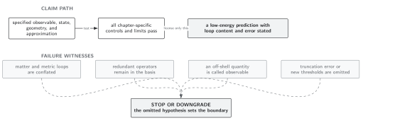
Momentum, curvature, species, coefficients, and duration must be varied independently; the first parameter reaching unity ends the associated expansion. The map is schematic and not to scale.

References

• Burgess, C. P. “Quantum Gravity in Everyday Life: General Relativity as an Effective Field Theory.” Living Reviews in Relativity 7, 5 (2004). doi:10.12942/lrr-2004-5. Open PDF
• Donoghue, J. F. “General Relativity as an Effective Field Theory: The Leading Quantum Corrections.” Physical Review D 50, 3874–3888 (1994). doi:10.1103/PhysRevD.50.3874. Open PDF