Euclidean Gravitational Saddles and Boundary Terms

A Euclidean gravitational saddle is defined by a differentiable action, boundary ensemble, regularity conditions, and an integration contour. The tunnelling exponent is the action difference from the false-vacuum reference at identical boundary data. A stationary metric obtained after dropping the Gibbons–Hawking–York term or changing the subtraction surface is not the same variational problem.

Required background. The gravitational-decay regime contract fixes the observable; flat-space bounces fixes the scalar boundary-value problem; and gravitational EFT power counting fixes omitted curvature operators.

Helpful background. Stokes jumps and saddle dominance supplies contour language, while proper-time and zeta determinants supplies the one-loop operator treatment.

The Dirichlet Euclidean problem

Set $\kappa=8\pi G$ and absorb the Euclidean cosmological term into

$$U(\phi)=V(\phi)+\frac{\Lambda_E}{\kappa}, \qquad \Lambda_E=-\Lambda_{\mathrm{site}}.$$

With $R_E=12H^2$ on a round four-sphere, use

$$S_E =\int_M d^4x\,\sqrt g \left[-\frac{R_E}{2\kappa} +\frac12(\nabla\phi)^2+U(\phi)\right] -\frac1\kappa\int_{\partial M}d^3x\,\sqrt h\,K +S_{\mathrm{ct}}.$$

The outward normal defines $K=h^{ij}\nabla_i n_j$. Holding $h_{ij}$ and $\phi$ fixed at the boundary makes the Einstein–scalar Dirichlet variation differentiable. If instead the ensemble fixes a conjugate momentum, the action must be Legendre transformed; a result from one ensemble cannot be compared with the other by subtracting the same number.

For a noncompact or regulated saddle, choose a cutoff surface in both the bounce and false reference, match the induced metric, scalar boundary value, and any Euclidean period, and only then take the cutoff away. Intrinsic counterterms must be identical functionals of the matched boundary data. Gibbons and Hawking show how the extrinsic-curvature term cancels the normal derivative in the Einstein–Hilbert variation (Gibbons and Hawking 1977, Eqs. (2.1)–(2.10)).

The structure map locates action and boundary data before the saddle equations and subtraction.

Dirichlet Euclidean saddle data. The diagram is schematic and not to scale; bulk equations, boundary variation, matched subtraction, and contour choice are independent checks.

O(4)-symmetric reduction

Take

$$ds_E^2=d\xi^2+\rho(\xi)^2d\Omega_3^2, \qquad \phi=\phi(\xi),$$

where the unit three-sphere has volume $2\pi^2$. The scalar curvature is

$$R_E =6\left[ \frac{1-\rho'^2}{\rho^2} -\frac{\rho''}{\rho}\right].$$

Substituting into the full action, integrating the $\rho''$ term once, and retaining the GHY contribution gives

$$S_E =2\pi^2\int d\xi\left\{ \rho^3\left(\frac12\phi'^2+U\right) -\frac{3}{\kappa}\rho(\rho'^2+1) \right\}.$$

This compact first-derivative form already includes the boundary cancellation. Its equations and Hamiltonian constraint are

$$\phi''+3\frac{\rho'}{\rho}\phi'=U_{,\phi},$$ $$\rho''=-\frac{\kappa\rho}{3}\left(\phi'^2+U\right), \qquad \rho'^2 =1+\frac{\kappa\rho^2}{3} \left(\frac12\phi'^2-U\right).$$

For a regular compact solution with two poles,

$$\rho(0)=\rho(\xi_{\max})=0, \quad \rho'(0)=1, \quad \rho'(\xi_{\max})=-1, \quad \phi'(0)=\phi'(\xi_{\max})=0.$$

These conditions make the boundary momenta vanish at the poles. For a finite outer boundary, variation of the reduced action leaves

$$\delta S_E\big|_{\partial M} =2\pi^2\left[ \rho^3\phi'\,\delta\phi -\frac{6}{\kappa}\rho\rho'\,\delta\rho \right]_{\partial M},$$

which vanishes under Dirichlet $\delta\phi=\delta\rho=0$. Deriving the reduced action from the bulk term alone gives a different boundary momentum and fails this check.

Using the constraint, the on-shell action can be written

$$S_E^{\mathrm{on}} =4\pi^2\int d\xi \left(\rho^3U-\frac{3\rho}{\kappa}\right).$$

For constant $U>0$, $\rho=H^{-1}\sin(H\xi)$ with $H^2=\kappa U/3$, and

$$S_E^{\mathrm{dS}}=-\frac{24\pi^2}{\kappa^2U}.$$

This constant-field check fixes every overall factor and the Euclidean curvature sign.

Boundary-term and subtraction adversarial test

Regulate a noncompact bounce at a surface of induced radius $\rho_B$ and its false reference at the same coordinate value rather than the same induced radius. The two boundary metrics then differ. Their leading volume and extrinsic-curvature pieces fail to cancel, so the apparent

$$B=S_E[\mathrm{bounce}]-S_E[\mathrm{false}]$$

depends on the regulator placement. Matching $\rho$, $\phi$, lapse normalization, and Euclidean period removes this artificial difference.

Now delete the GHY term while keeping Dirichlet data. The action variation contains normal derivatives of $\delta h_{ij}$, so a solution of the bulk equations is not stationary in the declared ensemble. Restoring GHY repairs differentiability. Adding an arbitrary finite boundary functional is allowed only if it represents a declared counterterm or ensemble change applied to both configurations.

Even after these repairs, the conformal-factor direction makes the real Euclidean metric integral unbounded. A decay interpretation needs a justified complex contour or steepest-descent cycle and the appropriate physical negative direction. Coleman and De Luccia’s scalar–gravity solutions supply saddle evidence within this framework, not a universal solution of the contour problem (Coleman and De Luccia 1980, §§ II–III).

The failure map separates a bad variational problem from a good saddle with an unresolved contour.

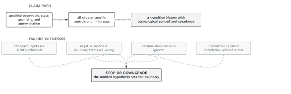
Failure conditions for a Euclidean gravitational saddle. The diagram is schematic and not to scale; differentiability and matched subtraction can be verified even when the full complex contour remains unresolved.

Domain and failure conditions

See the chapter domain and failure-conditions table. The reduction assumes four-dimensional Einstein gravity, a canonical scalar, O(4) symmetry, and either regular compact poles or a Dirichlet boundary with the displayed GHY term. Higher-curvature EFT operators require their own boundary completions and modify both the saddle and entropy-like on-shell terms.

Exercise

Derive the constant-field de Sitter action from the on-shell integral.

Solution

For $\rho=H^{-1}\sin H\xi$, $0\le\xi\le\pi/H$, and $U=3H^2/\kappa$,

$$S_E^{\mathrm{on}} =\frac{12\pi^2}{\kappa H^2} \int_0^\pi dx\, \left(\sin^3x-\sin x\right).$$

Since $\int_0^\pi\sin^3x\,dx=4/3$ and $\int_0^\pi\sin x\,dx=2$, the result is

$$S_E^{\mathrm{dS}} =-\frac{8\pi^2}{\kappa H^2} =-\frac{24\pi^2}{\kappa^2U}.$$

References

• Coleman, S., and F. De Luccia. “Gravitational Effects on and of Vacuum Decay.” Physical Review D 21 (1980): 3305–3315. DOI.
• Gibbons, G. W., and S. W. Hawking. “Action Integrals and Partition Functions in Quantum Gravity.” Physical Review D 15 (1977): 2752–2756. DOI.