Propagation of the Hadamard Property

Hadamard singularities do not have to be checked independently at every spacetime point. For a real, normally hyperbolic Klein–Gordon operator on a smooth boundaryless globally hyperbolic spacetime, the field equation transports the allowed null singularities. If a bisolution has the Hadamard relation on a neighborhood of one complete Cauchy surface, then it has that relation everywhere. This turns a local construction near initial data into a global ultraviolet result; it does not manufacture positivity or a state from arbitrary data.

Required background. Hadamard Admissibility and the Two-Point Wavefront Criterion states the directional condition. Green Functions and Causal Propagators supplies well-posed hyperbolic evolution.

Helpful background. Hyperbolic Equations and Causal Propagators develops the PDE setting. Singular Support and Wavefront Sets supplies the cotangent geometry.

The local-to-global theorem

Let $(M,g)$ be smooth, oriented, time oriented, globally hyperbolic, and without boundary. Let

$$P_\xi=\Box+m^2+\xi R$$

have real smooth coefficients and be formally self-adjoint. Its principal symbol is the Lorentzian quadratic form, so it is normally hyperbolic. Suppose $w\in\mathcal D'(M\times M)$ is a bisolution,

$$P_{\xi,x}w=P_{\xi,x'}w=0,$$

with the canonical antisymmetric part

$$w-w^{\mathsf T}=-iE, \qquad E=G_{\mathrm{ret}}-G_{\mathrm{adv}}.$$

Here $(x,k)\sim(x',k')$ means that one null geodesic contains $x$ and $x'$, the nonzero null covector $k$ has $k^\sharp$ tangent to that geodesic at $x$, and $k'$ is its parallel transport to $x'$. Let $\Sigma$ be a smooth spacelike Cauchy surface and let $N$ be an open neighborhood containing all of $\Sigma$. If the restriction of $w$ to $N\times N$ has the Hadamard wavefront relation, then

$$\operatorname{WF}(w) = \mathcal C^+ = \left\{ (x,k;x',-k'): (x,k)\sim(x',k'),\quad k\triangleright0 \right\}$$

on all of $M\times M$. Positivity is not needed to propagate this singularity statement. It is needed before $w$ may be called a state two-point function.

The historical local-parametrix result is the Fulling–Sweeny–Wald global singularity theorem Fulling, Sweeny, and Wald 1978, theorem and proof, pp. 259–264. A modern time-slice proof for state two-point functions is Khavkine and Moretti 2015, Proposition 16, pp. 50–51 (Open PDF); their Remark 23, pp. 51–52 (Open PDF) explains the extension to arbitrary bidistributions solving the field equation modulo smooth kernels and the partial-zero wavefront components that a naive proof misses.

The word Cauchy is essential. Hadamard form in an arbitrary small diamond controls only null rays that meet that diamond. A complete Cauchy surface meets every inextendible causal curve exactly once.

The three microlocal steps

For cotangent coordinates $(x,k)$, the principal symbol and Hamilton vector field are

$$p(x,k)=g^{ab}(x)k_a k_b,$$ $$H_p = \frac{\partial p}{\partial k_a}\frac{\partial}{\partial x^a} - \frac{\partial p}{\partial x^a}\frac{\partial}{\partial k_a}.$$

Three logically different facts enter:

1. Elliptic regularity confines singularities. For $P_\xi u=f$,

   $$\operatorname{WF}(u) \subset \operatorname{WF}(f)\cup\operatorname{Char}(P_\xi), \qquad \operatorname{Char}(P_\xi)=\{p=0\}.$$

   If $f$ is smooth, every remaining singular covector is null.

2. Hamilton flow transports them. Away from $\operatorname{WF}(f)$, the characteristic part of $\operatorname{WF}(u)$ is invariant under the maximally extended flow of $H_p$. For the homogeneous equation it is therefore a union of null bicharacteristics. Their projections are affinely reparametrized null geodesics, and their covectors are parallel transported. This is the real-principal-type propagation theorem Duistermaat and Hörmander 1972, §6.1, Theorem 6.1.1.

3. A time-slice reconstruction closes the two-point argument. Separate Hamilton propagation in the two slots explains the null geometry, but it is not by itself a complete proof: outside $N\times N$ it does not exclude product-cotangent elements $(x,k;x',0)$ or $(x,0;x',q)$. Choose $\chi_+$ to be zero sufficiently far to the past, one sufficiently far to the future, and to satisfy $\operatorname{supp}(\mathrm d\chi_+)\subset N$; put $\chi_-=1-\chi_+$. This partition is adapted to the Cauchy band. It defines a support-moving map

   $$\mathcal S f =f-P_\xi\!\left(\chi_+G_{\mathrm{adv}}f+\chi_-G_{\mathrm{ret}}f\right), \qquad \mathcal S:C_0^\infty(M)\longrightarrow C_0^\infty(N).$$

   Because $w$ is a bisolution, adding a $P_\xi$-exact test function in either slot changes nothing, so as distributional kernels

   $$w=\mathcal S^{\mathsf T}\circ (w|_{N\times N})\circ\mathcal S.$$

   The wavefront-set composition theorem, together with the known retarded and advanced Green-kernel relations, now transports the paired Hadamard cone and rules out the partial-zero components. The local relation fixes the future first-slot orientation; the canonical commutator supplies the physical antisymmetric normalization. This is the time-slice step in the proof of Khavkine and Moretti 2015, Proposition 16 and Remark 23, pp. 50–52 (Open PDF).

The lower-order terms $m^2+\xi R$ affect amplitudes and smooth tails, but not $p$. They cannot bend the characteristic cone or reverse a future-directed null covector.

What the Cauchy kernels determine

Let $n^a$ be the future unit normal to $\Sigma$ and define the Cauchy maps

$$\rho_0\phi=\phi\big|_\Sigma, \qquad \rho_1\phi=n^a\nabla_a\phi\big|_\Sigma.$$

Under the local Hadamard hypothesis near $\Sigma$, these pullbacks are well defined: the conormal covectors of a spacelike Cauchy surface are timelike, whereas the singular covectors of $w$ are null. Hyperbolic uniqueness then determines the bisolution from its four distributional Cauchy kernels

$$\lambda_{ij} = (\rho_i\otimes\rho_j)w, \qquad i,j\in\{0,1\}.$$

For a quasifree state, these kernels must jointly satisfy the induced CCR, Hermiticity, and positive-type inequality. Those are algebraic conditions on the initial covariance; they do not by themselves supply the Hadamard wavefront estimate. The present theorem addresses a different question: once the evolved bisolution has the Hadamard relation on a band $N$ around the complete surface, does that relation hold globally? The answer is yes.

Minkowski spacetime makes the transport explicit. With

$$p=k_0^2-\lvert\mathbf k\rvert^2,$$

Hamilton’s equations give

$$\dot t=2k_0, \qquad \dot{\mathbf x}=-2\mathbf k, \qquad \dot k_a=0.$$

Thus

$$x^a(\lambda)=x_0^a+2\lambda k^{\sharp a}$$

is a null line, and $k_0>0$ remains positive along it. Every inextendible line crosses the Cauchy surface $t=0$ and therefore every open band containing that surface. By contrast, a bounded diamond misses null lines sufficiently far away. Regularity inside that diamond says nothing about singularities on the missed lines.

The figure places these two tests side by side in logic but one above the other for narrow screens. In the upper panel every null orbit crosses the Cauchy band; in the lower panel a second orbit bypasses the controlled diamond.

On a narrow screen, swipe or use the Left and Right arrow keys to pan across the figure. Home and End move to its edges. A full-size link is also available.

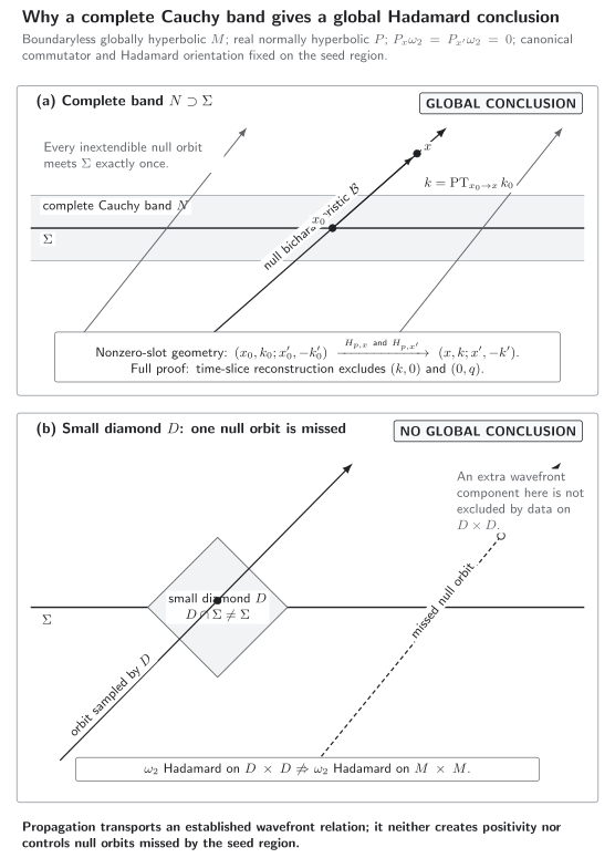
Complete Cauchy control versus a local patch. Solid null bicharacteristics crossing $N\supset\Sigma$ show why a complete Cauchy band reaches every orbit. The support-moving time-slice reconstruction in the text is still needed to control the full product wavefront set, including partial-zero covectors. A bounded diamond $D$ can be bypassed, so data on $D\times D$ cannot certify the missed orbit. Original schematic; not to scale. Semantic description (JSON).

What can start or hide a singularity

A nonsmooth source. For $P_\xi u=f$, propagation applies to $\operatorname{WF}(u)\setminus\operatorname{WF}(f)$. Singularities already present in $f$ can enter the characteristic flow. The source-free bisolution hypothesis is therefore substantive.

An incomplete patch. A small diamond can establish a local Hadamard statement, but not the global one. The missing null orbit in the figure is the negative control.

Loss of global hyperbolicity. There may be no complete Cauchy surface or unique global causal propagator. At base points of a compactly generated Cauchy horizon, an extended bisolution from an initial Hadamard state cannot differ from a local Hadamard distribution by a bounded function in any neighborhood Kay, Radzikowski, and Wald 1997, Theorem 2. This is a precise obstruction, not a generic claim about every non-globally-hyperbolic spacetime.

A different field operator. An unfixed gauge operator has a degenerate principal symbol and constraints. Losing normal hyperbolicity removes the license to invoke this scalar theorem; Dirac systems and suitably gauge-fixed Green-hyperbolic complexes require their own propagation results.

A timelike boundary. Boundary conditions determine reflected rays and boundary wavefront sets. The interior equation alone does not decide how singularities return from the boundary.

The strongest justified conclusion is correspondingly narrow: homogeneous normally hyperbolic evolution on the stated globally hyperbolic scalar domain propagates the Hadamard relation from a complete Cauchy neighborhood. Outside that domain, one needs a replacement theorem and additional data.

For the neighboring state claims and their failure conditions, see Domain and failure conditions.

Common pitfalls

Saying that propagation chooses the future cone. Hamilton flow preserves either time orientation. The local Hadamard condition chooses the future first-slot branch; propagation carries that choice.

Checking only a compact part of $\Sigma$. A neighborhood of a compact subset need not meet every inextendible null geodesic. The theorem needs an open neighborhood of the entire Cauchy surface.

Treating positivity as a PDE consequence. Hyperbolic evolution transports a covariance that is already positive, but the propagation-of-singularities theorem itself is not a positivity theorem.

Propagating the two slots separately and stopping. That argument follows components with nonzero covectors in both slots but does not rule out $(k,0)$ or $(0,q)$ components elsewhere on $M\times M$. The support-moving time-slice kernel and the composition theorem are the missing step.

Exercises

1. Lower-order terms. Why do $m^2$ and $\xi R$ not change the characteristic cone?

Solution

The characteristic set is the zero set of the principal symbol, which retains only the highest-derivative part of the operator. Both $m^2$ and $\xi R$ multiply the field without differentiating it, so the principal symbol remains $g^{ab}k_a k_b$ and its zero set is the null cone.

2. Minkowski Hamilton orbit. Integrate the Hamilton equations for $p=k_0^2-\lvert\mathbf k\rvert^2$ and verify that future orientation is preserved.

Solution

Because $p$ is independent of $x$, $\dot k_a=0$. Hence $k_a$ is constant and $x^a(\lambda)=x_0^a+2\lambda k^{\sharp a}$. On $p=0$ this curve is null. If $k_0>0$ initially, it remains positive because it is constant.

3. Singular source. Explain why the slogan “wavefront sets are unions of complete null bicharacteristics” needs qualification for $Pu=f$.

Solution

The theorem transports the source-free portion $\operatorname{WF}(u)\setminus\operatorname{WF}(f)$. At a covector in $\operatorname{WF}(f)$, the equation itself injects singular data, so a bicharacteristic component of $u$ may begin, end, or change there. The unqualified slogan is valid for $Pu\in C^\infty$, including $Pu=0$.

4. Three failed hypotheses. What survives if Hadamard form is known only in a small diamond, if the spacetime has a timelike boundary, or if it has a compactly generated Cauchy horizon?

Solution

In the diamond, only the local Hadamard conclusion and the null orbits reached from that patch are controlled. At a timelike boundary, propagation requires a boundary condition and a boundary-sensitive wavefront theorem. At a compactly generated Cauchy horizon, the globally hyperbolic theorem does not cross the horizon; at its base points the Kay–Radzikowski–Wald obstruction rules out a bounded difference from a local Hadamard distribution for an extended initial Hadamard bisolution.

5. The partial-zero gap. Why does propagating singularities in each variable separately fail to exclude $(x,k;x',0)$, and what feature of the time-slice proof repairs the problem?

Solution

For $P_{\xi,x}$, the product-space principal symbol depends only on the first covector $k$; for $P_{\xi,x'}$, it depends only on the second covector $q$. Ordinary propagation follows a characteristic component once the relevant slot covector is nonzero, but it does not turn a statement about such components into the absence of components whose other slot covector is zero. The identity

$$w=\mathcal S^{\mathsf T}\circ(w|_{N\times N})\circ\mathcal S$$

reconstructs the entire bidistribution from the Cauchy band. The kernel-composition theorem controls all product-cotangent components of that reconstruction, including the partial-zero projections, so none can appear outside the globally propagated Hadamard relation.

Handoffs

Constructing Hadamard States by Deformation and Gluing uses this theorem to transfer reference states through Cauchy evolution. Boundary and gauge cases begin with their own Green-hyperbolic analysis. The proof-level Hamilton-flow statement continues in Propagation of Singularities for Hyperbolic Fields.

References

• Duistermaat, Johannes J., and Lars Hörmander. “Fourier Integral Operators II.” Acta Mathematica 128 (1972): 183–269. DOI.
• Fulling, Stephen A., Mark Sweeny, and Robert M. Wald. “Singularity Structure of the Two-Point Function in Quantum Field Theory in Curved Spacetime.” Communications in Mathematical Physics 63 (1978): 257–264. DOI.
• Kay, Bernard S., Marek J. Radzikowski, and Robert M. Wald. “Quantum Field Theory on Spacetimes with a Compactly Generated Cauchy Horizon.” Communications in Mathematical Physics 183 (1997): 533–556. DOI. Open PDF.
• Khavkine, Igor, and Valter Moretti. “Algebraic QFT in Curved Spacetime and Quasifree Hadamard States: An Introduction.” In Advances in Algebraic Quantum Field Theory, 191–251. Cham: Springer, 2015. DOI. Open PDF.