Mode Matching Across Cosmological Eras

Mode matching transports canonical Cauchy data across a change in cosmological evolution. The reliable object is a symplectic transfer matrix—or the corresponding covariance map—not a particle number assigned at an artificial surface. A sharp junction is acceptable only as a controlled limit of resolved backgrounds or as an explicitly distributional model.

Required background. FLRW mode quantization fixes canonical data; conformal and minimally coupled scalars fixes the curvature potential; and adiabatic particle number fixes late-time interpretation. Helpful background. Review gravitational relic production for the abundance that consumes the transferred modes.

Canonical junction data

For $v_k''+\Omega_k^2v_k=0$, collect real canonical data in

$$z_k(\eta)= \begin{pmatrix}v_k(\eta)\\ v_k'(\eta)\end{pmatrix}, \qquad z_k(\eta_2)=T_k(\eta_2,\eta_1)z_k(\eta_1).$$

For a regular frequency, the fundamental matrix satisfies

$$T_k^{\mathsf T}JT_k=J, \qquad J=\begin{pmatrix}0&1\\-1&0\end{pmatrix}, \qquad \det T_k=1.$$

This identity is the real-data form of Wronskian preservation. It also transports a Gaussian covariance as $C_{k,2}=T_kC_{k,1}T_k^{\mathsf T}$, preserving the uncertainty bound. Multiplying era matrices preserves symplecticity, so determinant or Wronskian drift localizes an algebraic or numerical error.

The matched variables follow from the action, not from convenience. If $a$ is continuous but $a'$ has a declared jump at $\eta_*$, then $a''$ contains a delta distribution. Integrating the site scalar equation gives

$$v_k(\eta_*^+)=v_k(\eta_*^-), \qquad v_k'(\eta_*^+)-v_k'(\eta_*^-) =(1+6\xi)\frac{a'_+-a'_-}{a_*}v_k(\eta_*).$$

The conformal value $\xi=-1/6$ removes this kick, as it must. Imposing continuity of $v'$ for a minimally coupled scalar while retaining a delta in $a''$ would violate the distributional equation. Conversely, a smooth transition has no jump; its transfer matrix comes from ordinary evolution.

First application: de Sitter, reheating, radiation

Choose a quasi-de Sitter segment, a finite reheating interpolation, and radiation domination. Compute a fundamental matrix in each segment and form

$$T_k^{\rm total} =T_k^{\rm rad}T_k^{\rm reh}T_k^{\rm dS}.$$

Apply it to a normalized short-distance initial mode. Verify $\det T_k^{\rm total}=1$, the complex Wronskian remains $i$, and the transported covariance remains positive. Only in the late radiation regime, after an out basis has been declared, project the result to obtain $\alpha_k$ and $\beta_k$. Retaining the complex phase is essential: successive transitions interfere, so multiplying occupation numbers loses information.

Parker’s transfer between asymptotically stationary regimes makes clear that particle creation belongs to the complete evolution and its in/out bases Parker 1969, §§III–IV, pp. 1062–1067. A piecewise analytic approximation is therefore a method, not a physical claim by itself. Its uncertainty is estimated by varying junction locations and comparing with a resolved interpolation.

The structure map places the symplectic transfer before the late particle and relic branches. Inspect how canonical phase data cross every era.

Era matrices transport canonical data and covariance; Wronskian preservation survives their product, while particle number is assigned only in the stated out regime. Schematic; not to scale.

Domain and failure conditions

Use the chapter’s canonical domain table. State the differentiability of $a$, the canonical variable, whether distributional curvature is intended, the in/out bases, and the transition-resolution parameter.

Adversarial test. Replace every sharp junction by a family $a_\tau(\eta)$ that agrees away from a layer of width $\tau$ and converges in the declared topology. Evolve through the layer and compare phase, covariance, and late $\lvert\beta_k\rvert^2$ as the numerical grid resolves progressively smaller $\tau$. Reject an occupation or phase with no stable smooth-family limit. If the limit diverges because the proposed geometry carries unbounded curvature, the sharp model—not merely the solver—has left the effective description.

The failure map identifies mismatched variables, lost phases, and non-symplectic matrices before they contaminate an abundance. A controlled transfer can be handed to relic conversion or semiclassical backreaction together with the complex covariance and smoothing error; an artificial-junction spectrum cannot. Supplying only $\lvert\beta_k\rvert^2$ is insufficient whenever a later transition can interfere coherently with the transported state.

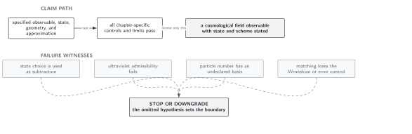
Canonical junction conditions, phase retention, symplecticity, and smooth-family convergence distinguish physical nonadiabatic evolution from artificial matching particles. Schematic; not to scale.

References

• Parker, L., “Quantized Fields and Particle Creation in Expanding Universes. I,” Physical Review 183, 1057–1068 (1969), doi:10.1103/PhysRev.183.1057.