Schwinger and Gravitational Production: A Controlled Comparison

Schwinger and gravitational particle production share a time-dependent oscillator equation and complex turning-point analysis, but they do not share all physical observables. Schwinger production depends on charge, gauge potential, electric work, and vacuum persistence. Gravitational production depends on the geometry, curvature coupling, state, and asymptotic time flow. Matching effective frequencies can match scalar Bogoliubov coefficients without equating currents, horizons, backreaction, or local stress tensors.

Required background. Particle Creation in Time-Dependent Backgrounds supplies in/out production; Adiabaticity, Stokes Phenomena, and Production Rates supplies turning-point control.

Helpful background. Gauge Fields, Gauge Fixing, and Ghosts on Curved Backgrounds supplies gauge structure; In–Out versus In–In Expectation Values separates vacuum persistence from real-time current.

Two effective frequency problems

For a charged scalar in a spatially homogeneous electric background $A_\parallel(t)$,

$$\ddot v_{\mathbf k} +\omega_{\mathbf k,E}^2(t)v_{\mathbf k}=0,$$

with

$$\omega_{\mathbf k,E}^2 = m^2+k_\perp^2 +\left(k_\parallel-qA_\parallel(t)\right)^2.$$

The gauge-invariant electric field is $E_\parallel=-\dot A_\parallel$. Canonical momentum $k_\parallel$ and kinetic momentum $k_\parallel-qA_\parallel$ must not be conflated.

For a scalar in four-dimensional spatially flat FLRW, the rescaled mode obeys

$$v_{\mathbf k}'' +\omega_{\mathbf k,g}^2(\eta)v_{\mathbf k}=0,$$

where

$$\omega_{\mathbf k,g}^2 = k^2+a^2m^2 +a^2(\xi-\xi_{\mathrm{conf}})R, \qquad \xi_{\mathrm{conf}}=-\frac16.$$

The two equations can be made mathematically identical for a selected mode profile. Their physical parameter maps, degeneracies, symmetries, and sources remain different.

For a constant electric field, the leading scalar mean occupation is

$$n_{\mathbf k} \sim \exp\!\left[ -\frac{\pi(m^2+k_\perp^2)}{\lvert qE\rvert} \right].$$

Schwinger’s effective-action result also determines vacuum persistence and its statistics-dependent sum over repeated tunneling events Schwinger 1951, pp. 664–679. The single-mode exponent is not the entire effective action.

First application: matched pulsed profiles

Choose a Sauter electric pulse and a solvable expanding background. To state an exact comparison, let $q(t)=\mathrm d\eta/\mathrm dt>0$, write the gravitational mode as $v(\eta(t))=\sqrt{q(t)}\,y(t)$, and require the two canonical frequencies to satisfy

$$\omega_{\mathbf k,E}^2(t) = q^2(t)\omega_{\mathbf k,g}^2(\eta(t)) +\frac12\frac{\ddot q(t)}{q(t)} -\frac34\left(\frac{\dot q(t)}{q(t)}\right)^2.$$

The last two terms are generated by the time reparameterization and field rescaling; omitting them generally changes the connection problem. If normalized in and out frequencies also match, the scalar connection problem gives the same $\lvert\beta_{\mathbf k}\rvert^2$.

The shared semiclassical data are:

• complex turning points $\omega^2=0$;
• actions $\int\omega\,\mathrm dt$;
• Stokes multipliers and saddle interference;
• the canonical identity $\lvert\alpha\rvert^2-\lvert\beta\rvert^2=1$.

The energy and observables differ. In the electric problem, produced charge sources a current and the external field does work,

$$\dot\rho_{\mathrm{pairs}} \supset \mathbf E\cdot\mathbf j.$$

In the expanding background, comoving mode energy is not generally conserved; the geometric source and stress conservation determine exchange. There may be no global timelike Killing energy during the production era.

Thus equality of $\lvert\beta\rvert^2$ for a matched scalar oscillator is a benchmark of the mode mathematics, not a proof that Schwinger and gravitational production are the same physical phenomenon.

Adversarial suppressed-data test

Erase $q$ and the distinction between $A_\mu$ and $F_{\mu\nu}$. The oscillator equation can still be written, but gauge transformations and the physical current can no longer be checked. Or copy a Schwinger exponent to an expanding spacetime without naming in/out states or a future time generator. The term called particle number then lacks its asymptotic definition.

Likewise, an acceleration horizon can yield detector KMS response without any charged pairs, while a finite electric pulse can create charged pairs without a causal horizon. Similar exponentials do not transfer horizon access, charge, spin-statistics factors, state preparation, or backreaction equations.

Construction and failure maps

The structure map identifies the shared middle layer—Bogoliubov or Stokes analysis—while retaining different states, backgrounds, observables, and energy sources on either side.

Matched effective frequencies benchmark the scalar production mathematics but do not identify the physical theories; the map is schematic and not to scale.

The failure map stops transfer of conclusions when charge, gauge invariance, horizon structure, state data, or the applicable asymptotic regime has been suppressed.

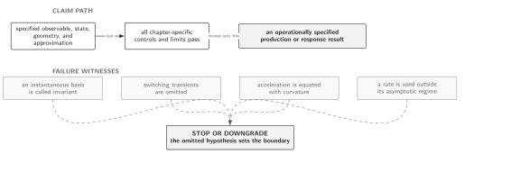
Only the matched oscillator coefficient and explicitly translated limits are shared; physical observables remain theory-specific. Schematic and not to scale.

Use the Stokes and energy rows in Domain and failure conditions. Report canonical versus kinetic momentum, gauge choice and invariants, curvature convention, state, asymptotics, turning points, prefactor and statistics, current or stress observable, source work, and backreaction parameter.

Check your understanding

If two mode equations have identical $\omega(t)^2$, which conclusion transfers automatically?

Solution

With matched normalization and asymptotic conditions, their scalar connection coefficients $\alpha$ and $\beta$ transfer. Charge current, gauge invariance, stress tensor, particle degeneracy, vacuum-persistence sum, detector response, and backreaction do not; they depend on structures outside the one-dimensional mode equation.

Detailed strong-field QED remains in the gauge-theory volumes, collapse and Hawking radiation in Chapter 6, and cosmological relic deployment in Chapter 14.

References

• Cesim K. Dumlu and Gerald V. Dunne, “The Stokes Phenomenon and Schwinger Vacuum Pair Production in Time-Dependent Laser Pulses,” Physical Review Letters 104 (2010), 250402, DOI, arXiv:1004.2509.
• Gerald V. Dunne, “Heisenberg–Euler Effective Lagrangians: Basics and Extensions,” in From Fields to Strings, World Scientific (2005), 445–522, DOI, arXiv:hep-th/0406216.
• Leonard Parker, “Particle Creation in Expanding Universes,” Physical Review Letters 21 (1968), 562–564, DOI.
• Julian Schwinger, “On Gauge Invariance and Vacuum Polarization,” Physical Review 82 (1951), 664–679, DOI.