Coupled State–Geometry Initial Data

Semiclassical initial data consist of more than a metric and a number called “vacuum.” One must specify geometric Cauchy data, a positive quantum state with Hadamard ultraviolet structure, finite renormalized gravitational couplings, compatible boundary data, and Hamiltonian and momentum constraints evaluated with that same state. These conditions prevent an initially finite but ultraviolet-inadmissible source from entering the coupled evolution.

Required background. The semiclassical Einstein equation fixes the sourced constraint; global hyperbolicity and Cauchy surfaces supplies the geometric initial-value setting; and constructing Hadamard states supplies admissible state data.

Helpful background. Propagation of the Hadamard property controls subsequent evolution, and stress-tensor ambiguities fixes the finite coupling data.

Geometric and quantum Cauchy data

Let $\Sigma$ be a compact Cauchy surface with future unit normal $n^\mu$. Write

$$g_{\mu\nu}=n_\mu n_\nu-h_{\mu\nu}, \qquad K_{ij}=-\frac12\mathcal L_n h_{ij},$$

where $h_{ij}$ is positive definite. The geometric data are $(h_{ij},K_{ij})$, modulo spatial diffeomorphisms, plus the finite values of $(\Lambda,G,a,b)$ and any boundary couplings.

For a quasifree scalar state, it is enough to give the four initial-surface distributions

$$W_{AB}(x,y) =\left. (n^\mu\nabla_\mu)^A (n^{\nu'}\nabla_{\nu'})^B W(x,y)\right|_{\Sigma\times\Sigma}, \qquad A,B\in\{0,1\}.$$

They must obey the field equation, Hermiticity, positivity, and the canonical antisymmetric part fixed by

$$W(x,y)-W(y,x)=-iE(x,y).$$

Because this chapter uses $E=G_{\rm ret}-G_{\rm adv}$ and $[\Phi(f),\Phi(h)]=-iE(f,h)$, the kernel convention must be checked rather than copied from an opposite definition of $E$. The symmetric part must have Hadamard wavefront set; equality of a few integrated moments is not enough. The propagation theorem then carries this singularity class through the globally hyperbolic development (Fulling, Sweeny, and Wald 1978, pp. 257–264).

With the conventions above, the local energy constraint is

$$\frac12\left({}^{(3)}R+K^2-K_{ij}K^{ij}\right) +\Lambda +a\,n^\mu n^\nu H^{(1)}_{\mu\nu} +b\,n^\mu n^\nu H^{(2)}_{\mu\nu} =8\pi G\,\rho_{\rm ren},$$

where $\rho_{\rm ren}=n^\mu n^\nu\langle T_{\mu\nu}\rangle_{\rm ren}$. The momentum constraint similarly equates $D_j(K^{ij}-h^{ij}K)$ to the renormalized momentum density, with higher-curvature terms included. If the unreduced equation is fourth order, additional geometric derivatives may be required; if order reduction is adopted, those data are deliberately excluded.

The structure map begins here: the state and geometry are one constrained datum, not independent inputs later adjusted to agree.

Initial data for the coupled problem. The diagram is schematic and not to scale; positivity, the canonical antisymmetric part, Hadamard singularities, finite couplings, and gravitational constraints are all imposed before evolution.

The failure map rejects ultraviolet tails that happen to have finite total energy. Failure of the Hadamard condition appears at the source and response stages even if the initial constraint can be assigned a finite number.

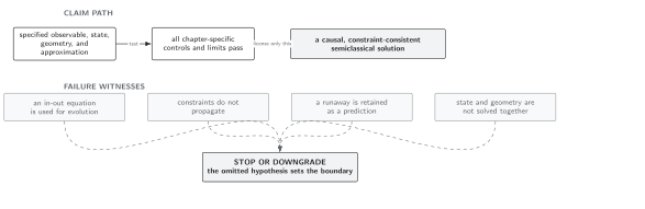
Ultraviolet admissibility test for state–geometry data. This schematic, not-to-scale map stops before a semiclassical solution is claimed when local composite fields, constraints, or state propagation are not well defined.

Application: Gaussian data on a three-torus

Take $\Sigma=T^3$ with coordinate volume $V$, $h_{ij}=a_0^2\delta_{ij}$, and $K_{ij}=-H_0h_{ij}$. Expand

$$\phi(t,\mathbf x)=\frac{1}{\sqrt V} \sum_{\mathbf k} \left[ a_{\mathbf k}\chi_{\mathbf k}(t)e^{i\mathbf k\cdot\mathbf x} +a_{\mathbf k}^\dagger\chi_{\mathbf k}^*(t)e^{-i\mathbf k\cdot\mathbf x} \right],$$

with initial mode data satisfying

$$a_0^3\left( \chi_{\mathbf k}\dot\chi_{\mathbf k}^* -\chi_{\mathbf k}^*\dot\chi_{\mathbf k} \right)=i.$$

A Gaussian state is fixed by these modes and nonnegative occupations $N_{\mathbf k}$, together with any allowed squeezing correlations. Choose fourth-order adiabatic large-$k$ data so that the stress subtraction is defined, and preferably an infinite-order Hadamard state when the response kernel will also be used.

For a minimally coupled illustration,

$$\rho_{\rm ren}(t_0) =\frac{1}{2V}\sum_{\mathbf k} (2N_{\mathbf k}+1) \left[ |\dot\chi_{\mathbf k}|^2+ \left(\frac{\mathbf k^2}{a_0^2}+m^2\right)|\chi_{\mathbf k}|^2 \right] -\rho_{\rm sub} +\rho_{\rm finite},$$

where curvature-coupling terms must be restored for $\xi\ne0$. The initial energy constraint reduces to

$$3H_0^2+\Lambda +aH^{(1)}_{00}(t_0)+bH^{(2)}_{00}(t_0) =8\pi G\,\rho_{\rm ren}(t_0).$$

One may solve this equation for $H_0$, a state parameter, or one finite coupling, but not all independently. Report which quantity was adjusted and verify the momentum constraint, which vanishes by homogeneity only if the state has no net momentum.

Adversarial test: a finite-energy non-Hadamard tail

Modify an otherwise Hadamard state by $N_k\sim k^{-6}$ at large physical momentum. In three dimensions its added energy behaves as

$$\Delta E\sim\int^\infty\!dk\,k^3N_k \sim\int^\infty\!dk\,k^{-3},$$

which converges. Nevertheless, the difference of two-point functions has only finite differentiability rather than being smooth; polynomial decay of all fixed order does not satisfy the Hadamard requirement. Higher local Wick products and metric response can expose the remaining singularity.

The strongest conclusion is that this tail defines finite energy in the chosen frame. It does not define admissible semiclassical initial data for all local observables and causal response. Replacing it by a rapidly decreasing smooth occupation or a verified Hadamard construction restores the claim.

Domain and failure conditions

See the chapter domain and failure-conditions table. This page assumes a boundary-free globally hyperbolic spacetime or boundary conditions with vanishing symplectic flux. It licenses evolution only after state positivity, CCR, Hadamard structure, finite couplings, and all gravitational constraints pass. A finite total energy, an instantaneous adiabatic label, or satisfaction of the Hamiltonian constraint alone is insufficient.

Exercise

Verify the homogeneous geometric part of the energy constraint.

Solution

For $K_{ij}=-H_0h_{ij}$,

$$K=-3H_0, \qquad K_{ij}K^{ij}=3H_0^2.$$

On the flat torus $^{(3)}R=0$, so

$$\frac12(K^2-K_{ij}K^{ij}) =\frac12(9-3)H_0^2 =3H_0^2.$$

This yields the displayed Friedmann constraint before higher-curvature and matter terms are added.

Handoff

In-in effective actions evolve these initial data with retarded memory rather than an in-out boundary-value prescription.

References

• Fulling, Stephen A., Mark Sweeny, and Robert M. Wald. “Singularity Structure of the Two-Point Function in Quantum Field Theory in Curved Spacetime.” Communications in Mathematical Physics 63 (1978): 257–264. DOI.
• Radzikowski, Marek J. “Micro-Local Approach to the Hadamard Condition in Quantum Field Theory on Curved Space-Time.” Communications in Mathematical Physics 179 (1996): 529–553. doi:10.1007/BF02100096.
• Wald, Robert M. Quantum Field Theory in Curved Spacetime and Black Hole Thermodynamics. Chicago: University of Chicago Press, 1994. Publisher record.