Euclidean and Bunch–Davies Free Fields in de Sitter

For a free scalar with positive effective mass, regularity on the Euclidean sphere selects a unique invariant Green function whose Lorentzian boundary value is the Bunch–Davies Wightman function. The statement depends on invertibility of the Euclidean operator, the analytic continuation, the canonical $i0$ boundary value, and the field algebra being considered.

Required background. de Sitter infrared regimes fixes the claim tuple; Bunch–Davies and alpha diagnostics fixes the state terminology; and FLRW mode quantization fixes the Wronskian. Helpful background. Review the Hadamard wavefront criterion.

The Euclidean two-point function

Let $Z(x,x')$ be the de Sitter invariant normalized so that $Z=1$ at coincidence. Choose any smooth dimensionless time function $T$ increasing to the future and define the Wightman boundary value

$$Z_\epsilon =Z-i\epsilon\,[T(x)-T(x')]-\epsilon^2, \qquad \epsilon\downarrow0.$$

For

$$M^2=m^2-12\xi H^2>0, \qquad \nu^2=\frac94-\frac{M^2}{H^2},$$

the four-dimensional Euclidean/BD Wightman function is

$$G^+(Z)=\frac{H^2}{16\pi^2} \Gamma\!\left(\frac32+\nu\right) \Gamma\!\left(\frac32-\nu\right) {}_2F_1\!\left( \frac32+\nu,\frac32-\nu;2; \frac{1+Z_\epsilon}{2} \right).$$

The oriented $i0$ is inherited from continuation through the appropriate complex-time tuboid; it is not chosen by de Sitter invariance alone. Different admissible time functions give the same distributional boundary value. The function solves $P_xG^+=0$ away from coincidence, its antisymmetric part has the site’s commutator sign $G^+(f,h)-G^+(h,f)=-iE(f,h)$ for $E=G_{\rm ret}-G_{\rm adv}$, and its coincidence singularity has the universal local Hadamard form.

In the expanding patch the same state is represented by

$$v_k^{\rm BD}(\eta) =\frac{\sqrt{-\pi\eta}}2 e^{i\pi(2\nu+1)/4}H_\nu^{(1)}(-k\eta),$$

with $v_kv_k^{*\prime}-v_k'v_k^*=i$. Its short-distance limit is $e^{-ik\eta}/\sqrt{2k}$. This normalization check fixes the distributional jump; matching only the hypergeometric differential equation would leave an overall coefficient and boundary value undetermined.

First application: continuation and restriction

Begin with the inverse of the positive elliptic operator on the Euclidean four-sphere and expand it in spherical harmonics. Continue the polar angle to global Lorentzian time, then take the Wightman boundary value. Three independent checks are available:

1. expand near $Z=1$ and match the local Hadamard pole;
2. restrict both points to the planar patch, Fourier transform spatially, and recover the Hankel modes and Wronskian above; and
3. take one point outside the planar patch in the global expression, showing that the global state exists even though one coordinate mode expansion does not cover both points.

Allen gives the invariant solutions and canonical normalization for the massive scalar Allen 1985, §§II–III, pp. 3138–3144. “Bunch–Davies” names the planar-patch mode representation of this Euclidean state; it is not a second state produced by restriction.

For the complementary series $0<M^2<9H^2/4$, $\nu$ is real and correlations decay slowly at large invariant separation. For the principal series, $\nu$ is imaginary and the decay oscillates. Neither slow decay nor a large light-mass amplitude violates the Hadamard condition, which constrains short-distance covectors rather than the infrared magnitude.

The structure map places Euclidean inversion, analytic continuation, canonical normalization, and patch restriction before any infrared resummation.

Euclidean regularity plus the Lorentzian boundary value fixes the standard massive free state; global and planar formulas are representations of the same two-point function. Schematic; not to scale.

Domain and failure conditions

The canonical domain table distinguishes this massive construction from the next page’s zero mode. The formula assumes the Euclidean inverse exists, a free scalar, exact de Sitter geometry, and the standard field algebra. Exceptional masses and gauge fields require their own zero-mode or constraint treatment.

Adversarial test. Add a de Sitter-invariant homogeneous bisolution proportional to the antipodal solution. It can preserve the field equation and formal symmetry, but constant negative-frequency mixing alters the short-distance boundary value and adds an antipodal singularity. Reject it as the standard state when Euclidean analyticity, the Hadamard wavefront condition, or local state-independent loop counterterms fail. Symmetry and a normalized commutator are necessary, not sufficient.

The validity map identifies the missing hypotheses before an invariant bisolution is called a physical vacuum. The $M^2\to0$ minimally coupled endpoint is handed to zero-mode analysis, not obtained by silently substituting zero into the massive inverse.

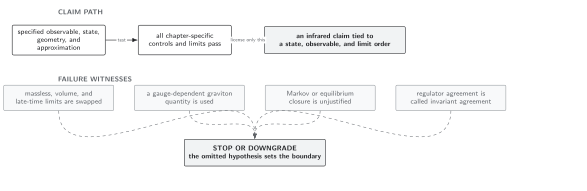
The field equation and de Sitter symmetry do not by themselves select the Euclidean/BD state; canonical boundary value and local singularity tests are decisive. Schematic; not to scale.

References

• Allen, B., “Vacuum States in de Sitter Space,” Physical Review D 32, 3136–3149 (1985), doi:10.1103/PhysRevD.32.3136.