

Correlation Extraction versus Causal Exchange on Curved Backgrounds
Two probes can become correlated because they sample correlations already present in the field, because one influences the other through the field, or because both mechanisms interfere. Curved spacetime makes the distinction especially important: a retarded tail can connect timelike supports after the direct null pulse has passed. The field anticommutator diagnoses state fluctuations; the commutator diagnoses causal exchange.
Required background. Causal Support, Signaling, and Global Geometry supplies the support test. Entanglement Harvesting in Curved Spacetime supplies the detector density matrix. Correlation Extraction versus Causal Exchange gives the abstract distinction.
Helpful background. Signaling, No-Signaling, and Causal Composition identifies sender-dependent influence. Entanglement Witnesses and Local Tomography Limits limits what detector data certify.
The covariance–commutator split
Section titled “The covariance–commutator split”For a real scalar field in state ,
where
The symmetric kernel depends on the state. The antisymmetric kernel is fixed by the free equation and causal boundary conditions. Smeared between causally disjoint supports, vanishes while generally does not.
Every second-order cross term in the two-detector state is linear in or its time-ordered version. It can therefore be written
with the pieces obtained by inserting and . The split is exact at this perturbative order once the same ordering prescription and detector profiles are kept. It does not imply that detector negativity is the sum of two negativities, because is nonlinear and interference between and can be constructive or destructive.
Three support regimes
Section titled “Three support regimes”Use the full detector worldtubes , not their central events.
Spacelike supports
Section titled “Spacelike supports”If and are causally disjoint, . Cross terms then come entirely from . If initially uncorrelated probes become entangled, “harvesting” is an appropriate description within the detector model. Local noise still competes with the extracted coherence.
Direct causal contact
Section titled “Direct causal contact”If , then may be nonzero. The sender can influence receiver statistics, and field-mediated interaction can generate entanglement even without sufficient pre-existing correlations. In flat-space massless detector fixtures this distinction can be quantitative and decisive Tjoa and Martín-Martínez 2021, §§ III–V. That result is model dependent: derivative couplings, masses, dimension, switching, or curvature can change the balance.
Tail-connected supports
Section titled “Tail-connected supports”The supports can be strictly timelike with no null-related pair yet still have through a curved-space tail. This is causal exchange. Calling it “vacuum harvesting” merely because the direct light-cone pulse is absent would be incorrect. The tail contribution is state independent for a free field, whereas the covariance contribution changes with .
A diagnostic calculation
Section titled “A diagnostic calculation”For each geometry and pair of detector supports, calculate:
where abbreviates switching, smearing, phase factors, and coupling. These norms are not themselves entanglement measures; they show which kernel is available. Then build four reduced states to the same perturbative order:
- the physical state with both contributions;
- the covariance-only diagnostic with cross-support set to zero;
- the exchange-only diagnostic with cross-support set to zero but physical local noise retained;
- a causally disjoint matched control.
The middle two are counterfactual decompositions, not necessarily completely positive standalone dynamics. Their purpose is to identify sensitivity, so report the physical density matrix and its positivity separately.
For spacelike, timelike, and tail-connected supports, evaluate the same negativity formula. A useful interference quantity is
Its sign states whether the two amplitudes reinforce or cancel in that matrix element. It is not an invariant allocation of entanglement to two independent resources. A 2026 de Sitter detector study explicitly finds expansion-dependent interference between communication and harvesting in causally connected models Zambianco, Teixidó-Bonfill, and Martín-Martínez 2026, §§ III–IV. As of August 2026 this is a theoretical detector-model result, not experimental confirmation of cosmological harvesting.
Turn off the commutator contribution
Section titled “Turn off the commutator contribution”The adversarial claim labels all final probe entanglement “harvested vacuum entanglement.” Apply the covariance-only diagnostic. If the negativity disappears, the original entanglement required exchange in that fixture and should be described as communication-generated or exchange-assisted. If it remains positive but changes, both mechanisms contributed. Only when the full supports are causally disjoint does microcausality remove the exchange ambiguity without a counterfactual decomposition.
This test also prevents the opposite error. A nonzero commutator does not prove that all final entanglement came from exchange; the covariance term may remain essential, and the two amplitudes can interfere.
Domain, limits, and maps
Section titled “Domain, limits, and maps”The canonical comparison is Domain and failure conditions. The decomposition is clean for free fields and perturbative linear detector couplings. At higher order, nested commutators, backreaction, and field-state changes complicate any allocation. Detector entanglement is an operational output of the chosen model, not a measure of the total entanglement initially present in local field algebras.
The structure map shows covariance and causal propagation entering before the joint detector metric. Inspect the commutator checkpoint whenever the supports are not spacelike.

Anticommutator correlations and commutator-mediated exchange can coexist and interfere; their sum feeds the physical detector state. Schematic; not to scale.
The failure map’s harvesting witness is the page’s adversarial test. Removing from the cross terms reveals whether the label survives.
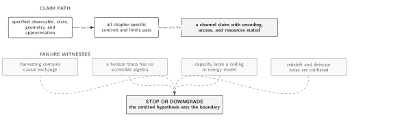
For timelike or tail-connected supports, final entanglement must be reported with its exchange sensitivity rather than called purely harvested. Schematic; not to scale.
Handoffs
Section titled “Handoffs”Causal Support, Signaling, and Global Geometry owns the retarded-tail analysis. Horizon-Restricted Local Operations and Distillability asks whether the resulting detector or field resource is accessible. General detector tomography belongs to Entanglement Witnesses and Local Tomography Limits.
References
Section titled “References”- Tjoa, Erickson, and Eduardo Martín-Martínez. “When Entanglement Harvesting Is Not Really Harvesting.” Physical Review D 104 (2021): 125005. DOI. Open PDF.
- Zambianco, Matheus H., Adam Teixidó-Bonfill, and Eduardo Martín-Martínez. “Cosmological Expansion Induces Interference between Communication and Entanglement Harvesting.” Physical Review D 113 (2026): 085023. DOI. Open PDF.
Original QFT.org content:CC BY 4.0, unless an item supplies different terms. Third-party material retains its own terms.