Gravitational Vacuum Decay and Cosmological Transitions

Vacuum decay with gravity and a cosmological first-order transition are not one calculation. A Euclidean saddle estimates an exponent for specified boundary data; a determinant and contour may turn that saddle into a decay rate; a real-time state defines a survival observable; a thermal rate is imported into an evolving expansion history; and completion, baryon yield, and gravitational-wave transfer are later, distinct inferences. This chapter keeps those layers separate and carries every supplied microscopic uncertainty into the cosmological output.

Helpful background. Flat-space bounce solutions and decay rates and negative modes supply the non-gravitational saddle machinery. Thermal nucleation rates supply microscopic plasma inputs, while FLRW field quantization fixes the expanding background.

Lorentzian and Euclidean data

With the site’s $(+---)$ metric and curvature convention, take the Lorentzian scalar–gravity action

$$S_L =\int_M d^4x\,\sqrt{-g}\left[ -\frac{R-2\Lambda_{\mathrm{site}}}{16\pi G} +\frac12g^{\mu\nu}\partial_\mu\phi\partial_\nu\phi -V(\phi)\right] -\frac1{8\pi G} \int_{\partial M}d^3x\,\sqrt{\lvert h\rvert}\, \epsilon K .$$

Here $n^\mu$ is outward pointing, $n^2=\epsilon=\pm1$, and $K=h^{\mu\nu}\nabla_\mu n_\nu$. The Einstein–Hilbert and GHY signs are the site signs: together with $T_{\mu\nu}=2(\sqrt{-g})^{-1}\delta S_m/\delta g^{\mu\nu}$ they give $G_{\mu\nu}+\Lambda_{\mathrm{site}}g_{\mu\nu}=8\pi G T_{\mu\nu}$. They differ from many mostly-plus references and must be translated as a pair.

After a declared Wick rotation and continuation of the metric, curvature tensor, cosmological term, and outward normal, the Euclidean action convention used here on a positive-definite metric is

$$\begin{aligned} S_E={}& -\frac1{16\pi G}\int_{M_E}d^4x\,\sqrt{g_E}\, (R_E-2\Lambda_E) \\ &+\int_{M_E}d^4x\,\sqrt{g_E}\left[ \frac12(\nabla_E\phi)^2+V(\phi)\right] -\frac1{8\pi G}\int_{\partial M_E}d^3x\,\sqrt h\,K_E +S_{\mathrm{ct}} . \end{aligned}$$

The Euclidean curvature convention is chosen so a round four-sphere has $R_E=12H^2$. For the corresponding constant-curvature continuation, $R_E=-R_{\mathrm{site}}$ and $\Lambda_E=-\Lambda_{\mathrm{site}}$; thus a positive scalar vacuum energy gives $H^2=(\Lambda_E+8\pi G V)/3$. The functional $S_E$ is obtained from the full site Lorentzian action by $e^{iS_L}\mapsto e^{-S_E}$, not by changing the signature while leaving individual curvature signs untouched. The Euclidean functional is not positive definite because its conformal metric direction is unbounded. The displayed Euclidean Gibbons–Hawking–York term is for fixed induced metric with the stated outward-normal convention. Compact regular instantons have no outer boundary. Noncompact saddles require reference subtraction or boundary counterterms, performed at matched induced boundary data. The decay exponent is never an absolute Euclidean action:

$$B=S_E[\text{saddle}]-S_E[\text{false-vacuum reference}]$$

in the same ensemble. Gibbons and Hawking derive the gravitational boundary term and thermodynamic action under fixed boundary geometry (Gibbons and Hawking 1977, Eqs. (2.1)–(2.10)).

The structure map shows the dependency chain. Saddle, fluctuation, real-time, thermal-history, and observational outputs occupy different stages.

From a metastable state to cosmological observables. The diagram is schematic and not to scale; each arrow requires its own state, ensemble, approximation, uncertainty, and failure test.

The failure map is the stopping rule. A stationary Euclidean point without the relevant contour and physical negative mode is saddle evidence, not yet a decay rate. One bubble per Hubble volume is a nucleation criterion, not percolation or completion. A supplied acoustic spectrum is a source model, not a present-day forecast until it has been propagated through a declared cosmology.

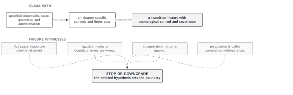
Failure conditions across gravitational decay and cosmological transitions. The diagram is schematic and not to scale; missing data stop the inference at the last controlled stage rather than being absorbed into an unexplained rate.

Route through the chapter

Order	Page and task
1	False-vacuum decay with gravity: fix the state, geometry, observable, hierarchy, and meaning of probability before choosing a method.
2	Euclidean gravitational saddles and boundary terms: pose a differentiable action and a matched action difference.
3	Coleman–De Luccia bounces: solve the inhomogeneous scalar–gravity saddle and continue its interior.
4	Hawking–Moss transitions and the stochastic crossover: compare homogeneous activation, inhomogeneous bounces, and coarse-grained diffusion only in their overlap.
5	Negative modes, determinants, and prefactors: reduce constraints and gauge before interpreting a determinant phase.
6	Real-time vacuum decay and state dependence: define survival as an initial-value observable on a closed time path.
7	Thermal nucleation in an expanding universe: integrate a supplied rate and equation of state without rederiving plasma microphysics.
8	Expansion history, percolation, and completion: distinguish first nucleation, connected converted volume, and disappearance of physical false-vacuum volume.
9	Baryogenesis inputs and the cosmological yield: propagate supplied CP sources and washout through reheating and entropy dilution.
10	Bubble sources and gravitational-wave propagation: separate source correlators from cosmological redshift and transfer.
11	Metastability, eternal inflation, and claim limits: separate local survival from volume weighting, measure choice, and quantum-gravity assumptions.

Domain and failure conditions

This is the chapter’s canonical comparison table. Every leaf links here and supplies its page-local assumptions.

Layer	Required input	Output or observable	Controlled statement	Decisive check	Failure or downgrade
Regime selection	Metastable state, background, region, clock, hierarchy	Proper-volume rate, survival probability, or history statistic	The chosen object has a definite operational meaning	Convert between rate and survival with the actual geometry	Treating foliation-dependent survival as an invariant local rate
Euclidean saddle	Euclidean action, boundary ensemble, contour candidate, matched reference	Action difference $B$	Stationary saddle evidence with declared boundary data	Vanishing boundary variation and invariant matched subtraction	Missing GHY term, unmatched reference, or unspecified conformal contour
Coleman–De Luccia	Scalar potential, gravitational coupling, regular pole data	Inhomogeneous bounce and Lorentzian bubble initial data	Controlled branch where a regular saddle exists	Numerical residual, constraint, thin-wall or weak-gravity limit	Continuing an exponent beyond branch disappearance
Hawking–Moss or stochastic	Barrier top, Hubble scale, coarse-graining, state	Homogeneous action difference or first-passage statistic	Overlap only under slow, light, Markovian, matched-observable conditions	Barrier-curvature scan and matched exponent limit	Calling two unlike observables identical or imposing a sharp universal crossover
Fluctuation rate	Gauge-reduced Hessian, measure, zero modes, contour	Prefactor multiplying $e^{-B}$	Decay interpretation when physical negative directions and determinant are controlled	Gauge and field-redefinition invariant spectrum	Conformal-factor, gauge, or extra-negative-mode ambiguity
Real-time decay	Initial density matrix, false sector, Hamiltonian, clock	$P_F(t)$ and time-dependent hazard	Initial-value result for the prepared state	State normalization, unitarity, and comparison in an exponential window	Universal rate inferred from the potential alone
Thermal nucleation	Versioned $\Gamma(T)$, covariance, equation of state	Nucleation-time or temperature distribution	Cosmological embedding of supplied microphysics	Reproduce adiabatic radiation limit and propagate covariance	Instantaneous equilibrium or rate precision unsupported by inputs
Percolation and completion	$\Gamma(t)$, $a(t)$, wall speed, reheating	False fraction, connected conversion, physical false volume	Separate nucleation, percolation, and completion times	Solve $P_F=e^{-I}$ and test $d(a^3P_F)/dt$	Declaring completion from one bubble per Hubble volume
Baryon yield	CP source, transport output, washout, entropy history	Final $Y_B=n_B/s$	Cosmological propagation of supplied charge microphysics	Time-variable and entropy-normalization invariance	Omitting washout, reheating, or entropy dilution
Gravitational waves	Unequal-time anisotropic-stress correlator, source lifetime, $a(t)$	Primordial and present-day spectra	Source calculation followed by cosmological transfer	Energy conservation, redshift, relativistic-degree count	Forecast precision below source-model or transfer uncertainty
Global self-reproduction	Local rate, patch dynamics, time variable, cutoff measure	Volume-weighted or first-passage statistic	Measure-conditional global statement	Repeat with declared time and cutoff prescriptions	Promoting a local rate to a measure-independent multiverse probability

A reproducible transition history

At minimum, preserve the supplied rate or source tables, their parameter definitions and covariance, the equation of state, wall and friction data, the expansion and temperature equations, entropy production, the numerical integration tolerances, and the definition of every event time. Report three separate stopping conditions:

$$\text{nucleation}, \qquad \text{percolation}, \qquad \text{completion}.$$

Then propagate only completed histories to a final yield or gravitational-wave spectrum. Coleman and De Luccia establish the gravitational-bounce framework (Coleman and De Luccia 1980, §§ II–IV); Guth and Weinberg give the expanding-background false-vacuum fraction that underlies the later history calculation (Guth and Weinberg 1983, Eqs. (2.1)–(2.8)).

References

• Coleman, S., and F. De Luccia. “Gravitational Effects on and of Vacuum Decay.” Physical Review D 21 (1980): 3305–3315. DOI.
• Gibbons, G. W., and S. W. Hawking. “Action Integrals and Partition Functions in Quantum Gravity.” Physical Review D 15 (1977): 2752–2756. DOI.
• Guth, A. H., and E. J. Weinberg. “Could the Universe Have Recovered from a Slow First-Order Phase Transition?” Nuclear Physics B 212 (1983): 321–364. DOI.
• Hawking, S. W., and I. G. Moss. “Supercooled Phase Transitions in the Very Early Universe.” Physics Letters B 110 (1982): 35–38. DOI.