Open-System Noise and Dissipation in de Sitter

Beyond the sharp-window leading limit, short modes act through both fluctuations and response. An influence functional retains colored noise, dissipation, initial correlations, and memory in one causal object. A white Markov Langevin equation follows only when the environment correlation time is short compared with every resolved long-field timescale and the coupling expansion remains controlled.

Required background. Stochastic coarse-graining fixes the moving split; influence functionals fixes the closed-time-path reduction; and noise, dissipation, and fluctuation relations fixes kernel conventions. Helpful background. Review non-Markovian memory and colored noise.

Influence kernels

Let a long variable $\phi$ couple through the declared plus-source convention $S_{\rm int}=+g\int\phi O$, and write $\delta O=O-\langle O\rangle$. With

$$\phi_c=\frac{\phi_++\phi_-}{2}, \qquad \phi_\Delta=\phi_+-\phi_-,$$

the second-order Gaussian influence action can be written

$$S_{\rm IF}= +\int dxdx'\,\phi_\Delta(x)D_R(x,x')\phi_c(x') +\frac{i}{2}\int dxdx'\, \phi_\Delta(x)N(x,x')\phi_\Delta(x').$$

Here the coupling is included in

$$D_R(x,x') =ig^2\theta(t-t')\langle[\delta O(x),\delta O(x')]\rangle, \qquad N(x,x') =\frac{g^2}{2}\langle\{\delta O(x),\delta O(x')\}\rangle.$$

Thus $D_R$ has retarded support and $N$ is the symmetric positive noise kernel. A Hubbard–Stratonovich field $\zeta$ with

$$\langle\zeta(x)\zeta(x')\rangle_\zeta=N(x,x')$$

turns the imaginary term into a generalized stochastic source. The mean equation then contains a causal memory integral,

$$\mathcal E[\phi](t) +\int_{t_0}^{t}dt'\,D_R(t,t')\phi(t') =\zeta(t).$$

Noise and dissipation are not interchangeable: $N$ controls fluctuations of histories, whereas $D_R$ changes their causal response. Dropping the latter while retaining the former generally violates the approximation order.

First application: a Gaussian short environment

Take $O=\chi_S^2/2$ with Gaussian short modes and interaction $g\phi_L\chi_S^2/2$. Wick’s theorem expresses both kernels through two short-mode propagators. Compute $N(t,t')$ from the anticommutator of $O$ and $D_R(t,t')$ from its retarded commutator, using the same window and initial state. Their width defines an environment correlation time $\tau_E$.

If

$$\tau_E\ll \tau_L, \qquad g^2\tau_E\ \text{is perturbative},$$

expand the long history inside the memory integral and approximate the noise by its integrated local strength. This yields local drift/damping and $N(t,t')\simeq2D(t)\delta(t-t')$, with $D$ defined by the integral of the colored kernel. Reverse the hierarchy, $\tau_E\gtrsim\tau_L$, and the derivative expansion ceases to be ordered: the colored kernel and initial slip must remain.

The influence-functional organization originates in the exact Gaussian-environment construction of Feynman and Vernon Feynman and Vernon 1963, §§II–IV, pp. 126–151. Applied to superhorizon scalar modes, an open-EFT derivation produces a Markovian Fokker–Planck limit together with leading corrections under a stated hierarchy Burgess et al. 2015, §§3–4, Eqs. (3.23)–(4.18).

A fluctuation–dissipation relation needs more. If the environment is stationary and KMS, the plus-source convention above gives $\rho(\omega)=2\operatorname{Im}D_R(\omega)$; then the symmetric kernel has the thermal form $N(\omega)=\tfrac12\coth(\beta\omega/2)\rho(\omega)$. A moving cosmological window is nonstationary and not generically KMS, even though a static-patch detector in the Euclidean state has a de Sitter temperature. Importing the static relation without matching time evolution is invalid.

The structure map places the influence kernels between QFT and any local stochastic reduction. Inspect the correlation-time comparison before the white-noise branch.

Colored noise and retarded response arise together; white Markov evolution follows only when the environment correlation time is parametrically shortest. Schematic; not to scale.

Domain and failure conditions

The chapter’s canonical domain table records the Markov and KMS hypotheses. The second-order action assumes weak coupling or a Gaussian environment truncation, a declared initial system–environment state, and causal in-in evolution. A moving split also requires boundary terms from modes crossing between sectors.

Adversarial test. First shrink $\tau_E/\tau_L$ while holding the integrated noise and retarded response fixed; verify that long correlators approach the local Markov solution. Then reverse the hierarchy and compare the full memory equation with the same local approximation. Require visible nonlocal deviations in the latter. If the local result persists only because $D_R$ or initial correlations were discarded, the test has not been performed.

Also propagate the reduced covariance and check the uncertainty bound. A finite-order master or Langevin truncation that drives the covariance nonpositive is not licensed as completely positive dynamics. The failure map sends long-memory problems to non-Markovian evolution and permits a thermal fluctuation–dissipation statement only after stationarity and KMS are demonstrated.

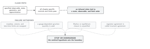
Markov, white-noise, thermal, and completely positive claims require separate correlation-time, response, KMS, and covariance checks. Schematic; not to scale.

References

• Burgess, C. P., R. Holman, G. Tasinato, and M. Williams, “EFT Beyond the Horizon: Stochastic Inflation and How Primordial Quantum Fluctuations Go Classical,” Journal of High Energy Physics 2015(03), 090 (2015), doi:10.1007/JHEP03(2015)090.
• Feynman, R. P., and F. L. Vernon Jr., “The Theory of a General Quantum System Interacting with a Linear Dissipative System,” Annals of Physics 24, 118–173 (1963), doi:10.1016/0003-4916(63)90068-X.