System–Environment Splits and Influence Functionals

An influence functional is the exact real-time record left by an environment after its variables have been integrated out. For a linearly coupled Gaussian environment it reduces to two kernels: a retarded kernel that changes propagation and a positive noise kernel that broadens fluctuations. The construction is exact only after the system–environment split and total initial state have been specified; locality, Markovianity, and a Lindblad generator require further approximations.

Required background. Open-system effective theory supplies the reduced-state construction, and closed-time-path generating functionals supply the doubled real-time contour. Helpful background. Real-time dissipative matching explains how retarded coefficients are extracted across scales.

From a microscopic trace to a doubled action

Take a system field $\phi$, environment variables $X$, and

$$S[\phi,X]=S_S[\phi]+S_E[X]-g\int_x\phi(x)\mathcal O_E(x).$$

For a factorized initial state $\rho_{SE}(t_0)=\rho_S(t_0)\otimes\rho_E$, the reduced density-matrix propagator contains a forward and a backward history. Integrating over $X_+$ and $X_-$ defines

$$e^{iS_{\mathrm{IF}}[\phi_+,\phi_-]} =\operatorname{Tr}_E\!\left( U_E[\phi_+]\rho_E U_E^\dagger[\phi_-] \right).$$

Equal histories cancel by unitarity,

$$S_{\mathrm{IF}}[\phi,\phi]=0,$$

which is the action form of trace normalization. Hermiticity gives

$$S_{\mathrm{IF}}[\phi_+,\phi_-]^* =-S_{\mathrm{IF}}[\phi_-,\phi_+].$$

These identities survive strong coupling and non-Gaussian environments. They do not, by themselves, prove complete positivity for an approximate action.

Introduce

$$\phi_r=\frac{\phi_++\phi_-}{2}, \qquad \phi_a=\phi_+-\phi_-.$$

If $\langle\mathcal O_E\rangle=0$ and the environment is Gaussian, the cumulant expansion terminates at second order. With the retarded self-energy $D_R$ and symmetrized kernel $N$ defined by the following action convention,

$$S_{\mathrm{IF}} =-\int_{x,y}\phi_a(x)D_R(x,y)\phi_r(y) +\frac{i}{2}\int_{x,y}\phi_a(x)N(x,y)\phi_a(y),$$

one has

$$D_R(x,y)=-ig^2\theta(x^0-y^0) \langle[\mathcal O_E(x),\mathcal O_E(y)]\rangle, \qquad N(x,y)=\frac{g^2}{2} \langle\{\mathcal O_E(x),\mathcal O_E(y)\}\rangle_c.$$

The sign multiplying $D_R$ changes if the interaction sign is changed; the causal support and the relation between the action and the equation of motion do not. The quadratic form $\int f^*Nf$ is nonnegative for Hermitian $\mathcal O_E$. It permits the Hubbard–Stratonovich representation

$$e^{-\frac12\phi_aN\phi_a} =\int\mathcal D\xi\,P[\xi]e^{i\xi\phi_a}, \qquad \langle\xi(x)\xi(y)\rangle_\xi=N(x,y),$$

so the same kernel appears as stochastic noise. This representation is exact for the Gaussian influence functional; a classical stochastic interpretation of every quantum observable is a stronger claim.

Thermal oscillator bath for one field mode

For one Fourier mode $q(t)$ coupled to oscillators $x_j$,

$$H_E=\sum_j\left(\frac{p_j^2}{2m_j}+\frac{m_j\Omega_j^2x_j^2}{2}\right), \qquad H_{\mathrm{int}}=-q\sum_jc_jx_j,$$

the spectral density

$$J(\Omega)=\frac{\pi}{2}\sum_j \frac{c_j^2}{m_j\Omega_j}\delta(\Omega-\Omega_j)$$

determines both kernels. The reduced equation is a generalized Langevin equation,

$$\ddot q(t)+\omega_{k,\mathrm{ren}}^2q(t) +\int_{t_0}^{t}ds\,\Gamma(t-s)q(s)=\xi(t), \qquad \langle\xi(t)\xi(s)\rangle=N(t-s).$$

$\Gamma$ is fixed by the retarded bath correlator. A local $q^2$ counterterm is generally required because the real part of the bath self-energy shifts the frequency. For a thermal state, the KMS condition relates $N(\omega)$ to the absorptive part of $D_R(\omega)$; noise and dissipation derives the precise relation.

An Ohmic Drude spectrum has the form

$$J(\Omega)\propto \Omega\frac{\Lambda^2}{\Omega^2+\Lambda^2}.$$

Its response kernel decays on the time $\Lambda^{-1}$. Replacing it by local damping is controlled only for system histories varying slowly compared with $\Lambda^{-1}$. Taking $\Lambda\to\infty$ before renormalizing the frequency shift conflates the memory approximation with the ultraviolet limit.

The oscillator-bath derivation and its initial-state subtleties are developed in Feynman and Vernon 1963, §§II–IV and the exact quantum Brownian-motion treatment of Hu, Paz, and Zhang 1992, §§II–III.

Initial correlations and the meaning of the split

Factorization at a finite $t_0$ is a physical assumption, not a harmless notation. Switching on a coupling suddenly can create an initial slip and cutoff-sensitive transient. A correlated thermal state of the interacting theory instead introduces contour correlations—often represented by an imaginary-time segment or explicit boundary vertices—and changes the reduced propagator.

For a fixed environment state and a factorized input, the exact map

$$\Phi_t(\rho_S)=\operatorname{Tr}_E[U_t(\rho_S\otimes\rho_E)U_t^\dagger]$$

is completely positive and trace preserving. With pre-existing correlations, a linear reduced map may be defined only on a compatibility domain of system states. It is then incorrect to demand or claim a CPTP extension without stating the preparation procedure.

The split itself is scale- and observable-dependent. A hard/soft mode division, a spatial subregion, and a particle/environment division retain different observables and produce different kernels. In a gauge theory the physical Hilbert space need not factorize across an arbitrary spatial boundary because Gauss constraints link the regions. One must choose a gauge-invariant operator algebra or introduce the appropriate edge or dressing data before tracing. None of these choices is uniquely fundamental.

Exact result, controlled approximation, or model

Keep three levels separate.

• An exact Gaussian trace fixes a nonlocal influence action for the declared bath and initial state.
• A perturbative cumulant expansion is controlled by coupling and correlation functions but need not remain positive after truncation.
• A phenomenological kernel can be useful if causality, noise positivity, normalization, and matching data are supplied, but it is not a microscopic derivation.

Before interpreting an influence action, check the tensor or algebraic split, initial preparation, environment state, coupling order, kernel regulator, counterterm convention, memory range, and normalization identity. Then test the approximate reduced map on more than the states used for matching. A reproducible calculation provides a bounded computational setting for such tests; a finite scan remains evidence on that setting.

Common failure modes

Inferring Markovianity from Gaussianity. A Gaussian bath makes the action quadratic, not local in time. Its spectral width controls memory.

Dropping the noise term. Keeping only the retarded self-energy can describe mean damping, but it does not reproduce reduced fluctuations and generally breaks the consistency of a quantum state.

Treating a factorized state as equilibrium. The product of the interacting system and bath Gibbs states is not the Gibbs state of the coupled theory.

Removing the cutoff before matching. Frequency shifts, local noise, and composite field jumps can require counterterms. State the regulator and renormalized parameters before taking a continuum limit.

This reduction map begins with the choices that control the entire calculation: the subsystem, the environmental variables, and their joint initial state.

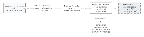
The first solid arrow is the environmental trace for the stated split and initial condition. The next arrow is not exact in general: a local master equation requires controlled memory and frequency approximations. The dashed branch identifies no-jump evolution as conditional rather than the full CPTP dynamics, and the final checks remain necessary even when the microscopic trace was exact. The diagram is schematic and not to scale.

Equivalently, the influence functional is the primary reduced object: its real and imaginary kernels encode response, fluctuations, and memory, including initial correlations. A Lindblad description is a further approximation whose error and regulator dependence must be stated rather than assumed.

Exercises

Show directly that $S_{\mathrm{IF}}[\phi,\phi]=0$ for a normalized environment state.

Solution

For equal histories, $U_E[\phi_+]=U_E[\phi_-]=U_E[\phi]$. Cyclicity of the trace and unitarity give $\operatorname{Tr}_E(U_E\rho_EU_E^\dagger)=\operatorname{Tr}_E\rho_E=1$. Hence $e^{iS_{\mathrm{IF}}[\phi,\phi]}=1$; choosing the branch continuous at zero coupling gives $S_{\mathrm{IF}}[\phi,\phi]=0$.

Suppose $N(t,s)$ has a negative eigenvalue as an integral kernel. Why can it not be the symmetrized correlator of a Hermitian Gaussian bath operator?

Solution

For any complex test function $f$, define $A=\int dt\,f(t)\mathcal O_E(t)$. The symmetrized covariance obeys $\frac12\langle A^\dagger A+AA^\dagger\rangle_c\ge0$. This is exactly the quadratic form $\int dt\,ds\,f^*(t)N(t,s)f(s)$. A negative eigenvalue therefore contradicts covariance positivity, although numerical discretization can create a spurious small negative value that should converge away.

Continue to local and nonlocal evolution

Quantum master equations label the Born, Markov, and secular steps that can turn these kernels into a time-local generator. Non-Markovian dynamics retains their finite-time tails, while open Schwinger–Keldysh actions organize the same information directly as field-theory vertices. Curved-spacetime and gravitational applications continue with influence-functional dissipation and noise.

References

• Breuer, Heinz-Peter, and Francesco Petruccione. The Theory of Open Quantum Systems. Oxford: Oxford University Press, 2002. doi:10.1093/acprof:oso/9780199213900.001.0001.
• Feynman, Richard P., and Frank L. Vernon Jr. “The Theory of a General Quantum System Interacting with a Linear Dissipative System.” Annals of Physics 24 (1963): 118–173. doi:10.1016/0003-4916(63)90068-X.
• Grabert, Hermann, Peter Schramm, and Gert-Ludwig Ingold. “Quantum Brownian Motion: The Functional Integral Approach.” Physics Reports 168 (1988): 115–207. doi:10.1016/0370-1573(88)90023-3.
• Hu, B. L., Juan Pablo Paz, and Yuhong Zhang. “Quantum Brownian Motion in a General Environment: Exact Master Equation with Nonlocal Dissipation and Colored Noise.” Physical Review D 45 (1992): 2843–2861. doi:10.1103/PhysRevD.45.2843.