Sources and Nonlinear Real-Time Response

Closed-time-path source derivatives generate causal response functions, not ordinary time-ordered amplitudes. At second order the answer is a sum of nested commutators over the two possible causal orderings of the perturbations, plus contact terms when the observable or Hamiltonian depends explicitly on the source.

Required background. Use the normalized contour functional and Keldysh causal diagrammatics.

Helpful background. Nonlinear response and higher Kubo relations develops transport limits and symmetry reductions.

Source convention and first response

Take

$$H_J(t)=H_0-J(t)O(t),$$

so the path-integral source is $+\int J\phi$ and the physical contour source is $J_a=0$, $J_r=J$. For an observable $A$ with no explicit source dependence,

$$R^{(1)}_{A;O}(t;t_1) \equiv\left.\frac{\delta\langle A(t)\rangle_J}{\delta J(t_1)}\right|_{J=0} =i\theta(t-t_1)\langle[A(t),O(t_1)]\rangle.$$

This sign follows directly from $H_J=H_0-JO$. With the chapter’s propagator convention $G^R=-i\theta\langle[O,O]\rangle$, the physical response for $A=O$ is $R^{(1)}=-G^R$. Many references choose the opposite source sign; comparing only the symbol $G^R$ is therefore insufficient.

In $r/a$ language, $\delta/\delta J_a$ inserts the measured $r$ field and $\delta/\delta J_r$ inserts an $a$ field. A response has one measured $r$ insertion and one $a$ insertion per physical-source derivative. The largest-time identity then guarantees that no perturbation acts after the measurement.

Second-order nested commutator

Expanding the interaction-picture evolution to second order, following the nested-commutator organization of Weinberg 2005, § III, gives

$$\begin{aligned} R^{(2)}_{A;OO}(t;t_1,t_2) =i^2\big[&\theta(t-t_1)\theta(t_1-t_2) \langle[[A(t),O(t_1)],O(t_2)]\rangle\\ &+\theta(t-t_2)\theta(t_2-t_1) \langle[[A(t),O(t_2)],O(t_1)]\rangle\big]. \end{aligned}$$

The two terms make the result symmetric under interchange of the identical source insertions, while each nested commutator has a definite causal ordering. There is no contribution if either $t_i>t$. This is not the three-point time-ordered correlator; the latter contains different operator orderings and is appropriate to in-out amplitudes or Euclidean continuation, not direct causal response.

For distinct perturbing operators $O_1,O_2$, retain their labels with the corresponding source derivatives. Frequency-space response also needs an explicit routing convention, for example $\omega=\omega_1+\omega_2$ into the measured operator. Losing the overall delta function or permuting an incoming frequency without its operator label creates false symmetry relations.

Contact and disconnected terms

If $A[J]$ depends explicitly on $J$, derivatives produce contact terms such as $\delta A/\delta J$. The same occurs when the Hamiltonian has a quadratic source coupling (“diamagnetic” or seagull term). Derivatives of step functions and derivative interactions can add equal-time commutators. These are required by Ward identities and cannot be discarded as coincident-point nuisances.

Using $W=-i\ln Z$ generates connected contour correlators. Differentiating $Z$ instead includes disconnected products; both are correct for their definitions, but mixing them double counts factorized pieces. State which functional is differentiated.

The dependency map makes explicit what functional differentiation does and does not remove. External sources select the response order, while the initial state, its boundary cumulants, and the finite-time memory kernel remain independent inputs to the observed response.

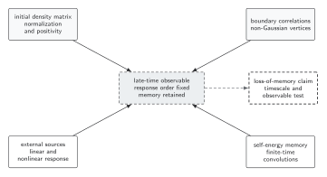
The arrows are a dependency map, not a causal-time orientation. Source derivatives generate linear and nonlinear response, but their retarded ordering, contact terms, and disconnected subtractions depend on the declared generating functional; initial correlations and memory are not thereby erased. The dashed branch permits a loss-of-memory statement only for a specified observable and separated timescale. The diagram is schematic and not to scale.

The sections Source convention and first response, Second-order nested commutator, and Contact and disconnected terms provide the text and equation equivalent of the source-to-response dependence.

Checked harmonic-oscillator examples

Let $A=O=q$ for a harmonic oscillator. Since $[q(t),q(t_1)]$ is a c-number, the second commutator vanishes, so

$$R^{(2)}_{q;qq}=0.$$

This matches the exact fact that the displacement of a linear oscillator is linear in the force. A nonzero numerical second-order response in this test indicates a source-routing, subtraction, or contact-term error.

For $A=q^2$ and $O=q$, the first commutator is operator valued, and the second nested commutator is generally nonzero. Thus nonlinear response can arise from the measured observable even when the Hamiltonian dynamics is Gaussian.

Equilibrium and nonequilibrium boundaries

Time-translation invariance reduces the number of independent time variables. KMS symmetry can further relate response and fluctuation functions, and microscopic time reversal can impose Onsager-type relations. Each step requires its own assumptions. The causal nested-commutator formula itself holds for an arbitrary initial density matrix; an equilibrium higher-order fluctuation relation does not.

Failure tests

• Reverse the source sign in a small exactly solvable model and verify the predicted odd/even response signs.
• Check that the result vanishes whenever a source time is later than the measurement.
• Compare source differentiation with direct finite differences of unitary evolution.
• Include explicit-source contact terms before testing a Ward identity.
• Route frequencies and operator labels together, and separate connected from full response.

Exercise

Show explicitly that the two terms in $R^{(2)}(t;t_1,t_2)$ make it symmetric under $t_1\leftrightarrow t_2$.

Solution

Interchanging $t_1$ and $t_2$ swaps the two displayed terms, including both step functions and nested-commutator labels. Their sum is unchanged. At $t_1=t_2$, the result depends on the declared equal-time and contact prescription.

Continue

For equilibrium reductions, combine this causal construction with KMS relations. For self-consistent two-time response, continue to nonequilibrium Green functions.

References

• Kubo, R. (1957). “Statistical-Mechanical Theory of Irreversible Processes. I.” Journal of the Physical Society of Japan 12, 570–586. DOI.
• Schwinger, J. (1961). “Brownian Motion of a Quantum Oscillator.” Journal of Mathematical Physics 2, 407–432. DOI.
• Weinberg, S. (2005). “Quantum Contributions to Cosmological Correlations.” Physical Review D 72, 043514. arXiv:hep-th/0506236; DOI.