Charged and Anomalous Hydrodynamics

An anomalous charge modifies hydrodynamics through a nonconservation equation and parity-odd magnetic and vortical response. The numerical coefficients depend on whether the current is consistent or covariant, on the Bardeen counterterm, on the hydrodynamic frame, and on whether the gauge field is a background or a dynamical variable. Only after those choices are fixed can a chiral magnetic or vortical coefficient be called observable.

Required background. Consistent and Covariant Anomalies fixes anomaly-current conventions. Local Equilibrium and Hydrostatic Constraints supplies the equilibrium functional.

Helpful background. Matrix-Valued Kinetics and Coherent Transport gives a microscopic transport route with Berry and coherence effects.

Current convention before constitutive data

Let $J^\mu_{\mathrm{cons}}$ be obtained by varying the generating functional. It satisfies the Wess–Zumino consistency condition but need not transform covariantly. Adding the local Bardeen–Zumino polynomial gives

$$J^\mu_{\mathrm{cov}} =J^\mu_{\mathrm{cons}}+J^\mu_{\mathrm{BZ}}[A,g].$$

The two divergences differ by a local source polynomial. To avoid hiding normalization, define the covariant $U(1)^3$ anomaly coefficient $C$ on this page by

$$\nabla_\mu J^\mu_{\mathrm{cov}} =C\,E_\mu B^\mu,$$

where

$$E^\mu=F^{\mu\nu}u_\nu, \qquad B^\mu=\frac12\epsilon^{\mu\nu\rho\sigma}u_\nu F_{\rho\sigma}, \qquad \epsilon^{0123}=+1.$$

Another source may place numerical factors in $C$ or use the consistent current. The Ward identity, not the letter assigned to its coefficient, is the translation key. Bardeen and Zumino derive the local polynomial relating the two current representatives Bardeen and Zumino 1984, §§2–4, pp. 421–435.

Hydrostatic magnetic response

On a stationary spatial slice, the parity-odd generating functional can contain

$$W_{\mathrm{odd}} = \frac12\int\mathrm d^3x\, \kappa(\mu,T)\epsilon^{ijk}A_i\partial_jA_k+\cdots.$$

For homogeneous $\kappa$, variation gives

$$J^i_{\mathrm{cons}}=\kappa B^i.$$

When $\kappa$ varies, its gradients generate additional magnetization and Bardeen–Zumino terms. Gauge variation of the complete hydrostatic functional must reproduce the chosen consistent anomaly; that requirement fixes the anomalous part of $\kappa$ and related vorticity terms. This is a response derivation, not an argument from entropy production alone Jensen, Loganayagam, and Yarom 2013, §§2–4, Open PDF.

The local covariant constitutive current has the parity-odd form

$$J^\mu_{\mathrm{cov}} =n\,u^\mu+\sigma_Q\mathcal V^\mu +\xi_B B^\mu+\xi_\omega\omega^\mu+\cdots.$$

In a commonly used thermodynamic or no-drag frame, the anomaly-dependent pieces are polynomial in $\mu$ and $T$; schematically, with coefficients normalized in that frame,

$$\xi_B=C\mu, \qquad \xi_\omega=\frac12C\mu^2+C_gT^2.$$

The mixed gauge–gravitational coefficient $C_g$ controls the indicated thermal term. A transformation to Landau frame adds terms proportional to $n/w$ times the anomaly-induced energy flow, so these simple component coefficients are not frame invariants. Son and Surowka derive the anomaly-constrained magnetic and vortical transport from the local second law, including the required frame corrections Son and Surowka 2009, pp. 1–4, Open PDF.

Equilibrium and transport are different limits

A hydrostatic magnetic current can include magnetization circulation. The transport current is obtained only after the subtraction and boundary prescription described on Contact Terms, Magnetization Currents, and Order of Limits. The limits

$$\lim_{\mathbf k\to0}\lim_{\omega\to0} \quad\text{and}\quad \lim_{\omega\to0}\lim_{\mathbf k\to0}$$

need not agree.

If the gauge field is dynamical, electric screening, Gauss constraints, and electromagnetic momentum must be included. A strictly conserved anomalous axial charge is also inconsistent without accounting for its anomaly; finite chirality-flipping and sphaleron rates move the chiral mode away from the origin. An equilibrium current in a compact sample is further constrained by boundary conditions and no-current theorems. None of these qualifications changes anomaly matching; they change which response is measured.

Collective-mode consequence

With a background magnetic field and a slowly relaxing axial/vector charge pair, anomaly-induced currents couple density perturbations along $\mathbf B$. A two-charge linear system has the schematic form

$$-i\omega \begin{pmatrix}\delta n_V\\ \delta n_A\end{pmatrix} +ikB \begin{pmatrix}0&v_{VA}\\v_{AV}&0\end{pmatrix} \begin{pmatrix}\delta n_V\\ \delta n_A\end{pmatrix} = - \begin{pmatrix}D_Vk^2&0\\0&\Gamma_A+D_Ak^2\end{pmatrix} \begin{pmatrix}\delta n_V\\ \delta n_A\end{pmatrix}.$$

For $\Gamma_A=0$, the reversible off-diagonal terms produce counterpropagating chiral magnetic waves; finite axial relaxation overdamps them at sufficiently small $k$. The velocities contain anomaly coefficients divided by susceptibilities, so the anomaly alone does not determine the observable dispersion.

Common pitfalls

Mixing consistent and covariant currents. Translate the Bardeen–Zumino term before comparing coefficients or Ward identities.

Calling a hydrostatic curl a transport current. Magnetization and boundary currents require explicit subtraction.

Using a background-field result for dynamical electromagnetism. Gauss law, screening, and electromagnetic stress change the slow sector.

Where this leads

Magnetohydrodynamics and Higher-Form Symmetries promotes magnetic flux to a dynamical hydrodynamic density. Sources, Linear Response, and Kubo Formulae fixes the retarded limit used to extract anomalous transport.

The anomalous-fluid branch is now distinct from the superfluid branch. Inspect its label “Ward identities + anomaly data”: anomalous transport modifies current constraints without requiring spontaneous symmetry breaking or a Goldstone phase.

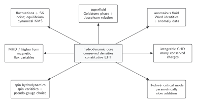
An anomalous fluid supplements ordinary hydrodynamics with anomalous Ward identities, consistent-versus-covariant current bookkeeping, and anomaly-matched constitutive data. It need not contain a Goldstone field; that belongs to the separate superfluid branch. The diagram is schematic and does not determine anomaly coefficients, equilibrium integration constants, or dynamical relaxation.

In text: declare the consistent anomaly, add the Bardeen–Zumino polynomial to obtain the covariant current when needed, impose hydrostatic and entropy constraints, and specify the order of zero-frequency and zero-momentum limits before calling a vortical or magnetic response transport.

References

• Bardeen, William A., and Bruno Zumino. 1984. “Consistent and Covariant Anomalies in Gauge and Gravitational Theories.” Nuclear Physics B 244: 421–453. DOI.

• Jensen, Kristan, R. Loganayagam, and Amos Yarom. 2013. “Thermodynamics, Gravitational Anomalies and Cones.” Journal of High Energy Physics 2013 (2): 088. DOI. Open PDF.

• Son, Dam T., and Piotr Surowka. 2009. “Hydrodynamics with Triangle Anomalies.” Physical Review Letters 103: 191601. DOI. Open PDF.