Conservation Laws and Hydrodynamic Fields

Relativistic hydrodynamics evolves expectation values of the stress tensor and conserved currents. A velocity field is introduced to decompose those observables into local energy, momentum, stress, charge, and spatial flux; it is not itself a uniquely defined microscopic observable away from equilibrium.

Required background. Current Sources and Generating Functionals derives currents by varying background sources. Spacetime Currents, Stress Tensors, and Charge Algebras fixes the stress-tensor and charge conventions used here.

Helpful background. Hydrodynamic Effective-Theory Architecture explains the derivative expansion that later closes these equations.

Source-covariant conservation laws

For a nonanomalous $U(1)$ current coupled to a background gauge field $A_\mu$ and a stress tensor coupled to $g_{\mu\nu}$,

$$\nabla_\mu J^\mu=0, \qquad \nabla_\mu T^{\mu\nu}=F^{\nu\lambda}J_\lambda, \qquad F_{\mu\nu}=\partial_\mu A_\nu-\partial_\nu A_\mu.$$

The second Ward identity includes the work and force supplied by the external field. In a local inertial frame its time component is the power density and its spatial components are the Lorentz-force density, once the displayed definition of $F_{\mu\nu}$ is used consistently. If the current is anomalous, if translations are explicitly broken, or if dynamical electromagnetism is included, the right-hand sides and field content must be changed rather than hidden inside a constitutive coefficient.

Decomposition relative to a velocity

Choose a future-directed unit timelike field $u^\mu$, $u^2=1$, and the positive rest-space metric $P^{\mu\nu}=u^\mu u^\nu-g^{\mu\nu}$. The most general symmetric stress tensor and current decompose as

$$\begin{aligned} T^{\mu\nu} &= \mathcal E u^\mu u^\nu +\mathcal P P^{\mu\nu} +u^\mu q^\nu+u^\nu q^\mu +\pi^{\mu\nu},\\ J^\mu &=\mathcal N u^\mu+j^\mu, \end{aligned}$$

with

$$u_\mu q^\mu=u_\mu j^\mu=0, \qquad u_\mu\pi^{\mu\nu}=0, \qquad \pi^\mu{}_{\mu}=0.$$

This irreducible decomposition and its relativistic-fluid interpretation are developed in Kovtun 2012, §2.1, pp. 15–21, Open PDF and Rezzolla and Zanotti 2013, ch. 2.

The scalars and fluxes are obtained directly from the physical tensors:

$$\mathcal E=u_\mu u_\nu T^{\mu\nu}, \quad q^\mu=T^{\mu\nu}u_\nu-\mathcal E u^\mu, \quad \mathcal N=u_\mu J^\mu, \quad j^\mu=J^\mu-\mathcal N u^\mu.$$

In the local rest frame, $T^{00}=\mathcal E$, $T^{0i}=q^i$, and $J^0=\mathcal N$. The spatial stress splits into its average $\mathcal P$ and traceless part $\pi^{ij}$. These relations are identities for any chosen $u^\mu$; hydrodynamics enters only when the components are expressed locally in terms of slow fields and sources.

Hydrodynamic frame and tensor reference

The table is the canonical convention and translation reference for Chapters 11–12. Every equality is in the site’s $(+---)$ convention; $d$ denotes spacetime dimension.

Object	Definition in this volume	Local-rest-frame or invariant check	Status under a first-order frame redefinition
Metric and velocity	$g_{\mu\nu}=\mathrm{diag}(1,-1,\ldots)$, $u^2=1$	$u^\mu=(1,\mathbf0)$	Convention fixed; $u^\mu$ itself is frame dependent
Rest-space metric	$P^{\mu\nu}=u^\mu u^\nu-g^{\mu\nu}$	$P^{ij}=\delta^{ij}$, $P^{\mu\nu}u_\nu=0$	Changes when $u^\mu$ changes
Derivatives	$D=u^\mu\nabla_\mu$, $\nabla_\perp^\mu=P^{\mu\nu}\nabla_\nu$	$D=\partial_t$, $\nabla_\perp^i=\partial_i$ at rest	Basis elements mix only at the next retained order
Expansion and acceleration	$\theta=\nabla_\mu u^\mu$, $a^\mu=Du^\mu$	$u\cdot a=0$	Frame dependent
Shear	$\sigma^{\mu\nu}=P^{\mu\alpha}P^{\nu\beta}(\nabla_\alpha u_\beta+\nabla_\beta u_\alpha+\tfrac{2}{d-1}P_{\alpha\beta}\theta)$	transverse and traceless; $\eta\sigma^{ij}$ is the usual negative viscous shear stress	Tensor coefficient $\eta$ is invariant at first order
Vorticity	$\omega^{\mu\nu}=\tfrac12P^{\mu\alpha}P^{\nu\beta}(\nabla_\alpha u_\beta-\nabla_\beta u_\alpha)$	transverse and antisymmetric	Not an independent parity-even first-order stress term
Stress and current	$T^{\mu\nu}=\mathcal E uu+\mathcal P P+2u^{(\mu}q^{\nu)}+\pi^{\mu\nu}$; $J^\mu=\mathcal N u^\mu+j^\mu$	reconstructing $T,J$ must give the original tensors	$T^{\mu\nu}$ and $J^\mu$ are invariant; components are not
Ideal data	$T_{(0)}^{\mu\nu}=\epsilon uu+pP$, $J_{(0)}^\mu=n\,u^\mu$	$w=\epsilon+p=Ts+\mu n$	Equation of state is invariant; its field coordinates change
Landau frame	$q^\mu=0$ through the chosen order	$u^\mu$ is the timelike energy-flow eigenvector when it exists	A matching convention, not an observable condition
Eckart frame	$j^\mu=0$ through the chosen order, requiring $n\ne0$	$u^\mu$ follows charge flow	Singular at $n=0$ and not automatically stable or causal
Invariant diffusion current	$\mathcal J^\mu=j^\mu-(n/w)q^\mu$	unchanged when $q\mapsto q-w\delta u$, $j\mapsto j-n\delta u$	Frame invariant through first order
Invariant scalar stress	$\mathcal B=\delta\mathcal P-p_\epsilon\delta\mathcal E-p_n\delta\mathcal N$	removes shifts along the equilibrium equation-of-state surface	Frame invariant through first order
Physical linear data	retarded poles, residues of fixed operators, Kubo coefficients	compute from $T,J$ correlators	Invariant through the consistently transformed truncation order

This is the chapter’s canonical translation table. Its scientific check is reconstruction: after any field redefinition, rebuild $T^{\mu\nu}$ and $J^\mu$ and verify equality through the retained derivative order.

Ideal variables and entropy

Local equilibrium supplies the zeroth-order functions

$$\mathcal E=\epsilon(T,\mu), \qquad \mathcal P=p(T,\mu), \qquad \mathcal N=n(T,\mu),$$

and the thermodynamic identities

$$\mathrm d\epsilon=T\,\mathrm ds+\mu\,\mathrm dn, \qquad \mathrm dp=s\,\mathrm dT+n\,\mathrm d\mu, \qquad w=Ts+\mu n.$$

The entropy current is not an additional exactly conserved microscopic current in a generic interacting theory. At ideal order $s^\mu=su^\mu$ follows from energy and charge conservation and obeys $\nabla_\mu s^\mu=0$ for smooth solutions. Dissipative corrections produce entropy and allow improvement ambiguities; the inequalities derived from them are treated on Onsager Reciprocity and Entropy Production.

Component check with an external field

In flat spacetime about rest, take $T^{00}=\epsilon$, $T^{0i}=wv^i$, and $J^\mu=(n,\mathbf J)$. The Ward identities reduce to

$$\partial_t\epsilon+\boldsymbol\nabla\!\cdot(w\mathbf v) =\mathbf E\!\cdot\!\mathbf J,$$ $$\partial_t(w\mathbf v)+\boldsymbol\nabla p =n\mathbf E+\mathbf J\times\mathbf B,$$

up to the order at which products of perturbations are retained. The first equation checks the sign of external work; the second checks that momentum of the matter sector alone is not conserved in a fixed electromagnetic background. If the electromagnetic field is dynamical, its stress tensor must be included so that the total stress is conserved.

Common pitfalls

Treating a decomposition as a constitutive law. Writing $T=\mathcal E uu+\cdots$ is kinematics. Predictive content starts only after the components are specified as functionals of the slow fields and sources.

Calling entropy an independently conserved charge. Entropy advection is an ideal, smooth-flow consequence. Dissipation, shocks, and fluctuations change the statement.

Forgetting improvements and magnetization. Local representatives of $T$ and $J$ can contain identically conserved pieces. Integrated charges and properly defined transport response remain the comparison targets.

Where this leads

Local Equilibrium and Hydrostatic Constraints determines which parts of these constitutive tensors follow from a stationary generating functional. Hydrodynamic Frames and Constitutive Data then derives the transformations summarized in the reference table.

The schematic places the Ward identities at the entrance to the constitutive construction. Inspect especially the dashed frame-change branch: it changes the fields used to decompose $T^{\mu\nu}$ and $J^\mu$, not those physical tensors themselves.

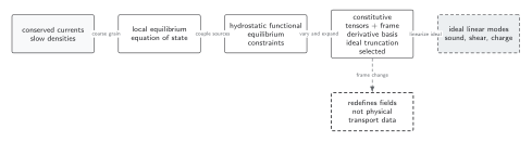
The physical inputs are the source-covariant conservation laws and the tensors $T^{\mu\nu}$ and $J^\mu$. Local equilibrium and hydrostatics constrain their constitutive form; a hydrodynamic frame only chooses coordinates on that form. The final mode box refers to the ideal-order truncation. The diagram is schematic and does not encode coefficient values or a causal initial-value theorem.

In text: decompose the fixed tensors relative to a chosen $u^\mu$, match $\epsilon$, $n$, $p$, energy flux, charge flux, and viscous stress, and translate those components order by order under field redefinitions. Ward identities and observable correlators survive that translation even though individual constitutive coefficients need not.

References

• Kovtun, Pavel. 2012. “Lectures on Hydrodynamic Fluctuations in Relativistic Theories.” Journal of Physics A: Mathematical and Theoretical 45: 473001. DOI. Open PDF.

• Rezzolla, Luciano, and Olindo Zanotti. 2013. Relativistic Hydrodynamics. Oxford University Press. DOI.