Infinite-Volume KMS States, Passivity, and Phase Multiplicity

In an infinite system the formal operator $e^{-\beta H}$ usually has infinite trace, so equilibrium cannot be defined by a global Gibbs density matrix. Instead a state is a positive normalized functional on a chosen algebra of local observables and is thermal when its time correlations satisfy the KMS analytic boundary condition. Different extremal KMS states at the same temperature encode distinct thermodynamic phases; their mixtures are equilibrium states but need not cluster.

The trace-free infinite-volume equilibrium framework is developed by Haag, Hugenholtz, and Winnink 1967, §§ 1–3, pp. 215–229.

Required background. Thermal Density Operators and the KMS Condition derives finite-volume KMS. Thermodynamic Limits, Phases, and Ensemble Equivalence fixes phase selection. Helpful background. Vacua, States, and Representations explains why inequivalent representations appear in infinite systems.

Local KMS without a global trace

Let $\mathfrak A$ be a unital $C^*$-algebra of quasilocal observables and $\alpha_t$ a strongly continuous one-parameter group of $*$-automorphisms. A state $\omega$ is a positive normalized linear functional,

$$\omega(A^*A)\ge0, \qquad \omega(\mathbf1)=1.$$

It is a $\beta$-KMS state if, for every $A,B\in\mathfrak A$, there is a function $F_{A,B}(z)$ analytic in $0<\operatorname{Im}z<\beta$, continuous and bounded on the closed strip, with boundary values

$$F_{A,B}(t)=\omega(A\alpha_t(B)), \qquad F_{A,B}(t+i\beta)=\omega(\alpha_t(B)A).$$

The placement of $A$ and $B$ differs from the previous page only by which operator is chosen as the time-translated one. The invariant content is the same cyclic imaginary-time boundary relation. An equivalent algebraic test can be made first on a norm-dense subalgebra of entire analytic elements and then extended by continuity. The algebra, dynamics, strip, and bounded observable class are part of the statement.

A thermodynamic-limit construction starts from a directed family of finite regions $\Lambda$ and local states $\omega_{\beta,\Lambda,b}$, where $b$ records the boundary condition or selecting source. Compactness can provide a weak-* convergent subnet; one may speak of a subsequence only when the relevant topology is metrizable. The finite-volume dynamics must also converge compatibly on local observables. The resulting functional is a candidate state, and one must still verify that the KMS boundary relation passes to the limit. Different choices of $b$ or of convergent subnet can select different phases.

Passivity as an operational equilibrium test

Let $\delta(A)=\left.\mathrm d\alpha_t(A)/\mathrm dt\right|_{t=0}$ generate the dynamics, and let $U$ be an admissible cyclic unitary in the domain of $\delta$. The work supplied to the system by that operation is

$$W_{\mathrm{on}}=-i\,\omega\!\left(U^*\delta(U)\right).$$

For finite-system dynamics $\delta(A)=i[H,A]$, this is $W_{\mathrm{on}}=\omega(U^*HU-H)$. A state is passive when $W_{\mathrm{on}}\ge0$ for every allowed cycle, equivalently when the extracted work $W_{\mathrm{ext}}=-W_{\mathrm{on}}$ is never positive Pusz and Woronowicz 1978, Definition 1.1, p. 276. It is completely passive if every finite tensor power is passive. In the same $C^*$-dynamical setting, KMS states at nonnegative inverse temperature and ground states are completely passive, and those are precisely the completely passive states under the theorem’s hypotheses Pusz and Woronowicz 1978, § 1, p. 278, Definition 1.3, Theorem 1.4, and the following remark.

Passivity is stronger than stationarity, but passivity alone does not imply KMS. The theorem’s $C^*$-dynamical-system setting, allowed operations, and tensor-product construction must be retained when exporting the complete-passivity classification. Passivity, Complete Passivity, and Ground States owns the theorem and its spectral proof.

Extremal phases, mixtures, and clustering

The convex set of $\beta$-KMS states may contain several extremal points. An extremal KMS state cannot be written as a nontrivial convex mixture of other KMS states at the same dynamics and temperature. In short-range systems, extremality is closely related to decay of connected correlations for suitable translated local observables,

$$\omega(A\,\tau_{\mathbf x}(B)) -\omega(A)\omega(B)\longrightarrow0 \qquad (\lvert\mathbf x\rvert\to\infty),$$

with hypotheses that depend on the algebra and translation action.

At coexistence, let $\omega_+$ and $\omega_-$ be symmetry-related extremal KMS states. Their mixture

$$\omega_{\mathrm{mix}}=p\,\omega_++(1-p)\omega_-$$

is also KMS because the condition is linear in the state. If an order parameter has values $\pm m$, however, the mixture has a nondecaying connected contribution $4p(1-p)m^2$. Thermal equilibrium therefore does not imply extremality or clustering.

Factorial KMS States, Phases, and Symmetry Breaking develops the hypotheses relating extremality, factoriality, and clustering.

The GNS representations $\pi_+$ and $\pi_-$ of distinct phases can be disjoint: they then share no nonzero unitarily equivalent subrepresentations. Equivalently, their normal-state folia obey

$$\mathcal F(\pi_+)\cap\mathcal F(\pi_-)=\varnothing,$$

so no state is normal in both representations. A trace-class density operator in one representation describes a state in that representation’s folium and cannot prepare a state in the disjoint folium. The stronger language of finite-energy local operations requires additional locality and energy hypotheses. States, GNS Representations, and Folia defines disjointness, while Local Normality, Quasiequivalence, and Folia separates local agreement from global phase inequivalence.

A controlled phase-selection statement

For a selected subnet $\{\Lambda_\iota\}$ with boundary condition $b$, a responsible infinite-volume claim has the form

$$\omega_b(A)=\lim_\iota\omega_{\beta,\Lambda_\iota,b}(A)$$

for every local $A$ in a specified convergence class. It then verifies KMS under the compatible limiting dynamics, identifies whether $\omega_b$ is extremal, and tests clustering or another phase criterion. Writing $\rho=e^{-\beta H}/Z$ after $Z$ has diverged skips every one of these steps.

Scope and theorem boundary

This page supplies the physics-facing definitions and consequences. Proofs of existence, uniqueness, decomposition, and equivalence between clustering and extremality depend on interaction range, locality, asymptotic abelianness, and topology. C*-Dynamical Systems and the KMS Condition owns the theorem-level formulation. The strongest safe conclusion here is conditional: a declared limiting state satisfying the KMS boundary condition is an equilibrium state for the declared dynamics, and multiple extremal such states represent phase multiplicity.

The upper panel separates the intrinsic KMS condition from the conditional construction of a local thermodynamic limit. Follow the dashed limit arrow, then compare the phase branch with the theorem-qualified complete-passivity branch.

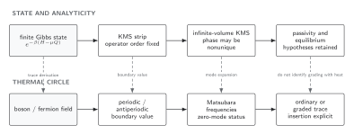
Finite trace cyclicity realizes the same positive-strip relation that defines an intrinsic KMS state. A thermodynamic-limit candidate reaches that condition only along a declared local subnet with compatible dynamics and a separate KMS check. Extremal phases and mixtures can coexist at one temperature, while complete passivity classifies KMS or ground states only under the Pusz–Woronowicz hypotheses; stationarity or passivity alone is insufficient. Dashed paths mark conditional constructions or hypotheses. The diagram is schematic and not to scale.

The lower Euclidean panel is included to show that a circle-mode representation is a separate gated consequence, not an automatic property of every algebraic KMS state.

Exercise

Suppose finite-volume states have been placed on one common quasilocal algebra and a subnet converges pointwise,

$$\omega(A)=\lim_\iota\omega_{\beta,\Lambda_\iota,b}(A).$$

Show that $\omega$ is positive and normalized. Explain why these facts alone do not prove that $\omega$ is KMS.

Solution

For scalars $c_1,c_2$ and observables $A_1,A_2$, pointwise convergence and finite-volume linearity give

$$\omega(c_1A_1+c_2A_2) =c_1\omega(A_1)+c_2\omega(A_2).$$

For any $A$, each finite-volume state also obeys $\omega_{\beta,\Lambda_\iota,b}(A^*A)\ge0$. Taking the pointwise limit preserves the inequality, so $\omega(A^*A)\ge0$. Likewise,

$$\omega(\mathbf1)=\lim_\iota \omega_{\beta,\Lambda_\iota,b}(\mathbf1)=1.$$

Thus $\omega$ is a state. KMS is stronger: one also needs a compatible limiting dynamics and sufficient control of the finite-volume analytic functions to pass analyticity, boundedness, continuity, and both boundary values to the limit. Pointwise convergence of real-time expectation values alone supplies none of those conclusions.

References

• Haag, Rudolf, Nico M. Hugenholtz, and Marius Winnink. “On the Equilibrium States in Quantum Statistical Mechanics.” Communications in Mathematical Physics 5 (1967): 215–236. doi:10.1007/BF01646342.
• Pusz, Wiesław, and Stanisław L. Woronowicz. “Passive States and KMS States for General Quantum Systems.” Communications in Mathematical Physics 58, no. 3 (1978): 273–290. doi:10.1007/BF01614224.

Further reading

• Ruelle, David. Statistical Mechanics: Rigorous Results. Singapore: World Scientific, 1999. doi:10.1142/4090.