Dynamic Universality Classes

Dynamic universality is determined by the complete infrared theory of slow variables: which order parameters are conserved, which additional densities remain slow, which reversible Poisson-bracket couplings symmetry allows, and whether momentum, long-range forces, or gauge fields participate. Two systems with identical static exponents can have different dynamic exponents and scaling functions.

Required background. Use static universality and scaling functions and dynamic scaling and critical slowing down.

Helpful background. Hydro+ and critical modes promotes an anomalously slow nonhydrodynamic mode into an extended fluid description.

The slow-variable classification

The classification logic of Hohenberg and Halperin 1977, §§ II–III requires a dynamic theory to list:

1. the order parameter, its symmetry representation, and static fixed point;
2. whether each component is exactly conserved;
3. conserved energy, momentum, charge, or other densities that remain slow;
4. reversible couplings fixed by Poisson brackets or commutators;
5. dissipative kinetic coefficients and noise required by detailed balance;
6. dimensionality, interaction range, and boundaries; and
7. every tuning that makes an otherwise fast mode parametrically slow.

Integrating out a genuinely slow density generates long memory and changes the universality class. Conversely, retaining a microscopic variable with finite relaxation rate need not change infrared exponents, though it can create a long crossover.

The schematic supplies a pipeline, not the class label. Selecting a dynamic universality class requires the complete slow-variable content, conservation laws, Poisson-bracket or reversible couplings, and equilibrium or nonequilibrium symmetry assumptions.

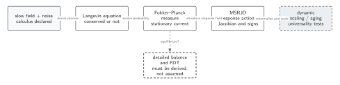
Models with the same static free energy can have different dynamic exponents because order-parameter conservation, additional conserved densities, and reversible couplings change the stochastic equations and response action. Noise color or amplitude alone does not select a class. The final scaling box is therefore conditional on a complete slow-variable classification and a stable dynamic fixed point. The diagram is schematic and not to scale.

The sections The slow-variable classification, Representative Hohenberg–Halperin models, and Reversible couplings and model dependence provide the text and equation equivalent of the model-selection conditions.

Representative Hohenberg–Halperin models

Selected dynamic universality classes and their distinguishing slow data

Model	Order parameter	Additional slow variables or couplings	Characteristic distinction
A	Nonconserved	No relevant conserved coupling	Pure relaxational dynamics; Gaussian $z=2$ before anomalous corrections
B	Conserved	No additional relevant slow field	Diffusive relaxation; conservation adds two powers of momentum
C	Nonconserved	Coupled conserved scalar density	Energy-like density can alter $z$ when the static specific-heat coupling is relevant
E/F/G	Multicomponent	Reversible couplings to conserved generators or second-sound variables	Propagating and precessional critical modes
H	Conserved scalar	Conserved momentum and advection	Liquid–gas or binary-fluid critical dynamics with mode coupling

These labels are hypotheses about the infrared theory, not names assigned by order-parameter appearance. Momentum conservation can be broken by a lattice, substrate, impurities, or external bath; energy can relax to an environment; long-range Coulomb interactions can gap a density mode. Each change can alter the class.

Checked Gaussian A versus B

For

$$\mathcal F=\frac12\int d^dx\,[r\phi^2+(\nabla\phi)^2],$$

Model A gives

$$\partial_t\phi=-\Gamma(r-\nabla^2)\phi+\xi,$$

so at criticality $\omega\sim-i\Gamma k^2$ and $z=2$.

For conserved Model B,

$$\partial_t\phi=\Gamma\nabla^2 \frac{\delta\mathcal F}{\delta\phi}+\nabla\cdot\boldsymbol\zeta,$$

so $\omega\sim-i\Gamma k^4$ and Gaussian $z=4$. The static functional is identical; conservation changes the dynamics. Interactions produce anomalous corrections but not the lesson.

Reversible couplings and model dependence

A term antisymmetric under interchange of slow variables can generate propagation without entropy production. Such reversible mode coupling is constrained by symmetry and Poisson brackets and can be relevant under dynamic RG. Dropping it because it vanishes in a static free energy misclassifies the dynamics.

Real systems can show crossover between classes when a nominally conserved density relaxes weakly. If its relaxation rate is $\gamma_b$, Model-H-like behavior may appear for frequencies above $\gamma_b$ and Model-A-like behavior below it. A single fitted $z$ over a narrow window can obscure this crossover.

Failure tests

• Verify conservation laws in the actual experimental or effective environment.
• Include all densities whose relaxation rate vanishes with $k$ or tuning.
• Derive reversible couplings from symmetry and brackets.
• Test interaction range, dimensionality, and momentum relaxation.
• Fit scaling over expanding size, frequency, and control-parameter windows.
• Compare at least two plausible classes when a bath relaxation scale is uncertain.

Exercise

Why does Model B have Gaussian $z=4$ rather than $z=2$?

Solution

Conservation forces the deterministic current to contain a gradient, so the evolution has an extra Laplacian: $\partial_t\phi=\Gamma\nabla^2(-\nabla^2\phi)$ at criticality. A Fourier mode decays as $\Gamma k^4$, hence $\tau_k\sim k^{-4}$ and $z=4$.

Continue

Apply the class-specific slow variables to generalized noise and quench, coarsening, and aging dynamics.

References

• Hohenberg, P. C., and Halperin, B. I. (1977). “Theory of Dynamic Critical Phenomena.” Reviews of Modern Physics 49, 435–479. DOI.