KMS Relations and Fluctuation–Dissipation

The fluctuation–dissipation relation is the frequency-space consequence of the KMS condition. Stationarity alone is insufficient: a driven steady state may depend only on time differences while its Wightman functions fail the imaginary-time KMS relation and therefore admit no universal thermal factor.

Required background. Use thermal density operators and KMS and the chapter’s causal/statistical conventions.

Helpful background. Detailed balance and stochastic fluctuation–dissipation gives the classical effective counterpart.

From KMS to Wightman functions

For a neutral bosonic operator in $\rho_\beta=e^{-\beta H}/Z$, the trace argument underlying Kubo 1957, §§ 2–3 gives

$$\langle O(t)O(0)\rangle_\beta =\langle O(0)O(t+i\beta)\rangle_\beta.$$

With $G^>(t)=-i\langle O(t)O(0)\rangle$ and $G^<(t)=-i\langle O(0)O(t)\rangle$, and Fourier transform $G(\omega)=\int dt\,e^{i\omega t}G(t)$,

$$G^>(\omega)=e^{\beta\omega}G^<(\omega).$$

Since $G^K=G^>+G^<$ and $G^R-G^A=G^>-G^<$,

$$G^K(\omega)=\coth\!\left(\frac{\beta\omega}{2}\right) [G^R(\omega)-G^A(\omega)]$$

for bosons on the nonzero-frequency sector: the equality is tested away from $\omega=0$, where the quotient is regular. The equivalent identity

$$G^R(\omega)-G^A(\omega) =\tanh\!\left(\frac{\beta\omega}{2}\right)G^K(\omega)$$

is meaningful also on a zero-frequency atom, but annihilates that atom and therefore cannot determine its weight. For fermions the antiperiodic KMS sign yields

$$G^K(\omega)=\tanh\!\left(\frac{\beta\omega}{2}\right) [G^R(\omega)-G^A(\omega)]$$

under the corresponding fermionic definitions. These compact formulas are convention sensitive; the Wightman ratio is the safest invariant starting point.

If $O$ carries charge $q$ and the state is $e^{-\beta(H-\mu Q)}$, the thermal factor becomes $\omega-\mu q$, provided $[Q,O]=-qO$ under the declared sign convention. Pairing charged conjugate operators matters: applying a neutral formula to $OO$ when the nonzero correlator is $OO^\dagger$ is an error. For a charged bosonic pair, the singular point of the coth quotient is correspondingly $\omega-\mu q=0$ and must be resolved before division.

KMS appears only in the final, explicitly conditional box of the contour schematic. The contour and $r/a$ basis exist for arbitrary normalized initial states; thermal analyticity is the extra hypothesis that closes spectral and statistical information into a fluctuation–dissipation relation.

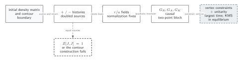
Unitarity and largest-time identities constrain every normalized closed-time-path theory, while KMS additionally requires a thermal state and time-translation-invariant equilibrium dynamics. The diagram’s quadratic-inversion step applies to the two-point propagators; thermal vertex relations require the separately rotated interaction and KMS symmetry. Under the equilibrium hypotheses, KMS relates Wightman functions and hence the spectral and statistical correlators. Stationarity alone does not justify the last relation. The diagram is schematic and not to scale.

The sections From KMS to Wightman functions and Why stationarity is not KMS give the text and equation equivalent of the equilibrium hypothesis, derived relation, and failure boundary.

Classical and zero-frequency limits

For nonzero $|\beta\omega|\ll1$,

$$\coth(\beta\omega/2)=\frac{2T}{\omega}+O(\omega/T).$$

Thus low-frequency fluctuations are enhanced relative to dissipation. The apparent $1/\omega$ singularity must be treated with the spectral measure or specified regulated distribution. A limit of ordinary spectral densities and a delta function at exactly zero are different objects; absence of an atom alone does not define multiplication of an arbitrary distribution by the singular coth factor.

The distinction is explicit for a Hermitian observable in a finite-dimensional Gibbs system. Use connected correlators by replacing $O$ with $\delta O=O-\langle O\rangle_\beta$. If $P_E$ projects onto the full energy eigenspace, including degeneracy, set

$$O_0=\sum_E P_E\delta O P_E, \qquad C_0=\langle O_0^2\rangle_\beta\ge0.$$

Equal-energy matrix elements contribute the same amount to the two Wightman measures. Consequently,

$$G_c^K(\omega)=-4\pi i C_0\delta(\omega)+G_{c,\ne0}^K(\omega), \qquad (G^R-G^A)\big|_{\{0\}}=0.$$

Here $G_{c,\ne0}^K$ denotes the part supported away from zero. Centering removes the mean but leaves a conserved thermal variance. In particular, if $[H,O]=0$, then $C_0=\operatorname{Var}_\beta(O)$, the entire connected noise is static, and the commutator response vanishes. A complete reconstruction of the noise therefore needs both the nonzero-frequency FDT relation and $C_0$. The full projector, not just a chosen matrix diagonal, is needed when energy levels are degenerate.

This is the invariant contribution singled out by Kubo 1957, § 3, pp. 576–577, Eqs. (3.12), (3.15)–(3.17). For $H-fO$, re-equilibration at fixed temperature gives the imaginary-time susceptibility $\chi_T=\int_0^\beta d\lambda\,\langle\delta O(-i\lambda)\delta O(0)\rangle_\beta$. It need not equal the isolated retarded susceptibility at zero frequency; for a conserved observable the former is $\beta C_0$ and the latter is zero. The solved finite-spin example includes both conserved and oscillating components and translates the raw-noise convention into this page’s $-i$ convention. In continuum QFT, use suitably smeared operators with finite moments or a specified renormalized/regulator limit before extending the finite spectral argument.

For a free oscillator, $G^R-G^A$ has peaks at $\omega=\pm\omega_0$. Multiplication by $\coth(\beta\omega/2)$ gives weights $2n_B(\omega_0)+1$, exactly reproducing $G^K$. This checks the sign at both positive and negative frequency.

Why stationarity is not KMS

A density matrix diagonal in the energy basis is stationary, but unless its weights have the Gibbs form—or generalized chemical potentials associated with the operator algebra—its Wightman ratio is not $e^{\beta\omega}$ with a single $\beta$. A periodically driven steady state, generalized Gibbs ensemble, or mode-dependent Gaussian state can likewise be stationary without ordinary KMS.

Defining

$$\coth\!\left(\frac{\omega}{2T_{\mathrm{eff}}(\omega)}\right) =\frac{G^K}{G^R-G^A}$$

is only a parametrization when the ratio is well defined. A physical effective temperature requires a frequency window, operator independence, positive thermodynamic interpretation, and consistency with independent observables. One fitted ratio does not establish thermalization.

Failure tests

• Test the Wightman KMS ratio directly, including the operator charge and chemical-potential shift.
• State the Fourier sign; reversing it changes which exponential appears.
• Vary the frequency window and operator before quoting an effective temperature.
• Resolve zero-frequency distributions and contact terms before taking limits.
• Do not impose KMS on a driven or aging state merely because a late-time correlator looks stationary over a short interval.

Exercise

Starting from $G^>=e^{\beta\omega}G^<$, derive the bosonic $\coth$ factor on the nonzero-frequency sector. Explain why this does not reconstruct the connected noise of a conserved Hermitian observable with nonzero thermal variance.

Solution

Write $G^K=(e^{\beta\omega}+1)G^<$ and $G^R-G^A=(e^{\beta\omega}-1)G^<$. Away from zero, the first multiplier equals the second times $\coth(\beta\omega/2)$, giving the stated relation without dividing by the spectral measure itself. For a conserved centered observable, $G_c^>=G_c^<=-2\pi i\operatorname{Var}_\beta(O)\delta(\omega)$. Hence $G^R-G^A=0$ while $G_c^K=-4\pi i\operatorname{Var}_\beta(O)\delta(\omega)$. The zero of the KMS multiplier erases this weight, which must be retained separately.

Continue

Use nonlinear response for higher source derivatives. In a general nonequilibrium state, evolve $F$ and $\rho$ independently rather than imposing this relation.

References

• Callen, H. B., and Welton, T. A. (1951). “Irreversibility and Generalized Noise.” Physical Review 83, 34–40. DOI.
• Kubo, R. (1957). “Statistical-Mechanical Theory of Irreversible Processes. I.” Journal of the Physical Society of Japan 12, 570–586. DOI.
• Martin, P. C., and Schwinger, J. (1959). “Theory of Many-Particle Systems. I.” Physical Review 115, 1342–1373. DOI.