Unruh Temperature and Thermal Periodicity

The previous page rewrote ordinary Minkowski two-point functions in Rindler coordinates. A striking fact appeared immediately: when both points lie in the right wedge, the Minkowski Wightman function has an analytic continuation whose boundary values are related by an imaginary shift of Rindler time. This page explains why that KMS relation, rather than naive pointwise periodicity, is the defining structure of thermal equilibrium.

The route is deliberately indirect. We first review thermal correlators in ordinary quantum mechanics and field theory, because the Unruh effect is not a mysterious new kind of heat; it is the Kubo–Martin–Schwinger condition applied to the boost Hamiltonian. We then connect the KMS condition to detailed balance, Euclidean time circles, Matsubara frequencies, and fluctuation–dissipation. Finally we apply the same logic to a uniformly accelerated detector and obtain

$$\boxed{T_U={a\over 2\pi}}.$$

Here $a$ is the detector’s proper acceleration, and $k_B=\hbar=c=1$. The result says that the Minkowski vacuum, restricted to the algebra of observables accessible to one uniformly accelerated observer, behaves as a thermal state with respect to that observer’s proper-time evolution.

Required background. Rindler coordinates and Green functions supplies boost time, wedge localization, and the Minkowski Wightman function in accelerated coordinates.

Helpful background. In–out, in–in, and Schwinger–Keldysh functionals distinguishes amplitudes from expectation values, while proper time, determinants, and thermal traces introduces Euclidean traces and periodic paths.

Thermal correlators and the KMS condition

Thermal-time conventions. For an operator $A$ in the Heisenberg picture,

$$A(t)=e^{iHt}Ae^{-iHt}.$$

A thermal expectation value at inverse temperature $\beta$ is

$$\langle \mathcal O\rangle_\beta={1\over Z}\operatorname{Tr}\left(e^{-\beta H}\mathcal O\right), \qquad Z=\operatorname{Tr}e^{-\beta H}.$$

For Rindler time we write

$$\eta=a\tau,$$

where $\tau$ is proper time along the worldline $\rho=1/a$. The inverse temperature conjugate to dimensionless boost time $\eta$ is $\beta_R=2\pi$. The inverse temperature conjugate to proper time $\tau$ is therefore

$$\beta={2\pi\over a}.$$

Let

$$C^>_{AB}(t)=\langle A(t)B(0)\rangle_\beta, \qquad C^<_{AB}(t)=\langle B(0)A(t)\rangle_\beta.$$

The two functions are not generally equal. Their difference is a commutator and controls response; their sum is noise. Thermal equilibrium relates them by a complex-time shift.

Using

$$A(t-i\beta)=e^{\beta H}A(t)e^{-\beta H},$$

we find

$$C^>_{AB}(t-i\beta) ={1\over Z}\operatorname{Tr}\left(e^{-\beta H}e^{\beta H}A(t)e^{-\beta H}B(0)\right).$$

Cancel the first two exponential factors and then use cyclicity of the trace:

$$C^>_{AB}(t-i\beta) ={1\over Z}\operatorname{Tr}\left(A(t)e^{-\beta H}B(0)\right) ={1\over Z}\operatorname{Tr}\left(e^{-\beta H}B(0)A(t)\right).$$

Therefore

$$\boxed{ C^>_{AB}(t-i\beta)=C^<_{AB}(t). }$$

Equivalently,

$$\boxed{ \langle A(t)B(0)\rangle_\beta = \langle B(0)A(t+i\beta)\rangle_\beta. }$$

This is the KMS condition. It is the analytic definition of thermal equilibrium. For bosonic operators it often looks like periodicity in imaginary time, but the precise statement is stronger and more careful: shifting by $-i\beta$ changes the operator ordering.

The trace manipulation is literal for a finite system with a trace-class Gibbs operator. In continuum QFT, the thermodynamic limit may not admit a density matrix of the form $Z^{-1}e^{-\beta H}$ on the vacuum Hilbert space. The intrinsic statement is then that the correlators are boundary values of functions analytic in the KMS strip and obey the same boundary relation. This is the form needed for wedge-local quantum fields.

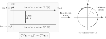
The KMS condition says that a thermal Wightman function has analytic continuation in a strip of height $\beta$. The lower edge is the oppositely ordered correlator. In Euclidean language, the same information becomes a thermal circle of circumference $\beta$.

For a single bosonic operator $J$, define

$$G^>(t)=\langle J(t)J(0)\rangle_\beta, \qquad G^<(t)=\langle J(0)J(t)\rangle_\beta.$$

Then KMS gives

$$G^>(t-i\beta)=G^<(t).$$

For a time-translation-invariant thermal state, $G^<(t)=G^>(-t)$ if $J$ is Hermitian. Thus a common one-operator form is

$$G^>(t-i\beta)=G^>(-t).$$

This is exactly the form that appears for the Minkowski vacuum restricted to a Rindler wedge.

Detailed balance from spectral sums

The KMS condition becomes especially physical after a Fourier transform. Take a Hermitian operator $J$ and insert a complete set of energy eigenstates,

$$H|n\rangle=E_n|n\rangle.$$

With the convention

$$G^>(\omega)=\int_{-\infty}^{\infty}dt\,e^{i\omega t}G^>(t),$$

we obtain

$$G^>(\omega) ={2\pi\over Z}\sum_{m,n}e^{-\beta E_m}|J_{mn}|^2 \delta\left(\omega-(E_n-E_m)\right).$$

The same calculation gives

$$G^<(\omega) ={2\pi\over Z}\sum_{m,n}e^{-\beta E_m}|J_{mn}|^2 \delta\left(\omega-(E_m-E_n)\right).$$

Relabeling $m\leftrightarrow n$ in the second expression yields

$$G^<(\omega)=e^{-\beta\omega}G^>(\omega).$$

For a Hermitian operator, $G^<(\omega)=G^>(-\omega)$, so

$$\boxed{ G^>(-\omega)=e^{-\beta\omega}G^>(\omega). }$$

This is detailed balance. Processes related by reversing the direction of energy flow differ by the Boltzmann factor.

For a two-level detector with gap $\Omega>0$, weak coupling and stationary long-time evolution give the Golden Rule rates

$$\Gamma_\uparrow=\lambda^2|\mu_{eg}|^2\mathcal F(\Omega), \qquad \Gamma_\downarrow=\lambda^2|\mu_{eg}|^2\mathcal F(-\Omega),$$

where

$$\mathcal F(\Omega)=\int_{-\infty}^{\infty}ds\,e^{-i\Omega s}G^+(s).$$

The KMS condition implies

$$\boxed{ {\Gamma_\uparrow\over\Gamma_\downarrow}=e^{-\beta\Omega}. }$$

Equivalently, for a bosonic oscillator mode of frequency $\Omega$,

$$\Gamma_\uparrow\propto n(\Omega), \qquad \Gamma_\downarrow\propto 1+n(\Omega),$$

with

$$\boxed{ n(\Omega)={1\over e^{\beta\Omega}-1}. }$$

The $1$ in $1+n$ is spontaneous emission; the $n$ term is stimulated emission. Equilibrium is the condition that upward and downward transitions balance after including the Boltzmann weights of the detector states.

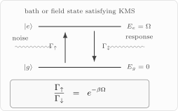
A two-level detector in a thermal bath has upward and downward transition rates related by detailed balance. The ratio $\Gamma_\uparrow/\Gamma_\downarrow=e^{-\beta\Omega}$ is the operational content of temperature.

This is the right language for acceleration. An accelerated detector does not infer temperature by reading a coordinate label. It infers temperature because its transition rates obey detailed balance with a definite $\beta$.

Euclidean time circle and Matsubara modes

Thermal traces can be written as Euclidean path integrals. For a bosonic coordinate $q$, the matrix element of $e^{-\beta H}$ is an imaginary-time transition amplitude. Taking the trace identifies the endpoints, so

$$Z(\beta)=\operatorname{Tr}e^{-\beta H} =\int_{q(\beta)=q(0)}\mathcal Dq\,e^{-S_E[q]}.$$

For a scalar field,

$$Z(\beta)=\int_{\phi(\tau_E+\beta,\mathbf x)=\phi(\tau_E, \mathbf x)}\mathcal D\phi\,e^{-S_E[\phi]}.$$

Fermions are antiperiodic rather than periodic,

$$\psi(\tau_E+\beta, \mathbf x)=-\psi(\tau_E, \mathbf x),$$

because the trace over fermionic states and coherent-state variables produces an extra sign.

For bosons, the allowed Euclidean frequencies are

$$\boxed{ \omega_n={2\pi n\over\beta}, \qquad n\in\mathbb Z. }$$

For fermions,

$$\boxed{ \omega_n={2\pi\left(n+{1\over2}\right)\over\beta}, \qquad n\in\mathbb Z. }$$

As the simplest example, consider a harmonic oscillator of frequency $\omega_0$. Its Euclidean thermal Green function satisfies

$$\left(-{d^2\over d\tau_E^2}+\omega_0^2\right)G_E(\tau_E)=\delta_\beta(\tau_E),$$

where $\delta_\beta$ is the periodic delta function on the circle. Therefore

$$\boxed{ G_E(\tau_E) ={1\over\beta}\sum_{n\in\mathbb Z} {e^{i\omega_n\tau_E}\over \omega_n^2+\omega_0^2}. }$$

For $0\le \tau_E\le \beta$, the same answer can be written as

$$\boxed{ G_E(\tau_E) ={1\over2\omega_0} {\cosh\left[\omega_0\left({\beta\over2}-|\tau_E|_\beta\right)\right] \over \sinh\left({\beta\omega_0\over2}\right)}, }$$

where $|\tau_E|_\beta$ means the shortest distance to $0$ on the thermal circle. In the zero-temperature limit $\beta\to\infty$, the sum becomes an integral and

$$G_E(\tau_E)\to {1\over2\omega_0}e^{-\omega_0|\tau_E|}.$$

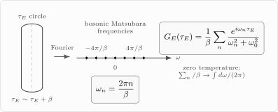
A thermal trace becomes a Euclidean path integral on a circle of circumference $\beta$. Bosonic fields are periodic and therefore have Matsubara frequencies $\omega_n=2\pi n/\beta$.

The connection with Rindler space is now almost visible by inspection. Euclidean Rindler time is an angle. If the geometry is smooth at the origin, that angle must have period $2\pi$. Thermal periodicity is therefore built into the regularity of the Euclidean plane.

Fluctuation–dissipation

Thermal field theory distinguishes two real-time questions. One asks how much the system fluctuates in equilibrium. The other asks how the system responds to a small external perturbation.

For a Hermitian operator $J$, fluctuations mean connected correlations: write $\delta J=J-\langle J\rangle_\beta$ and

$$G_c^>(t)=\langle\delta J(t)\delta J(0)\rangle_\beta, \qquad G_c^<(t)=\langle\delta J(0)\delta J(t)\rangle_\beta.$$

The following spectral sums are literal for a finite-dimensional Gibbs system. In QFT, use suitable smeared operators with finite thermal moments or a specified regulator and renormalized correlation distributions. Centering leaves the commutator unchanged, so define

$$\rho(\omega)=G_c^>(\omega)-G_c^<(\omega) =\int_{-\infty}^{\infty}dt\,e^{i\omega t} \langle[J(t),J(0)]\rangle_\beta,$$

and the symmetrized noise

$$S_c(\omega)={1\over2}\left(G_c^>(\omega)+G_c^<(\omega)\right) ={1\over2}\int_{-\infty}^{\infty}dt\,e^{i\omega t} \langle\{\delta J(t),\delta J(0)\}\rangle_\beta.$$

Using

$$G_c^<(\omega)=e^{-\beta\omega}G_c^>(\omega),$$

we get

$$\rho(\omega)=\left(1-e^{-\beta\omega}\right)G_c^>(\omega),$$

and

$$S_c(\omega)={1\over2}\left(1+e^{-\beta\omega}\right)G_c^>(\omega).$$

An identity that remains meaningful on a zero-frequency spectral atom is

$$\boxed{ \rho(\omega)=2\tanh\left({\beta\omega\over2}\right)S_c(\omega). }$$

On the nonzero-frequency sector, division gives the familiar fluctuation–dissipation relation,

$$S_c(\omega)={1\over2}\coth\left({\beta\omega\over2}\right)\rho(\omega), \qquad \omega\ne0.$$

Here the restriction means equality of spectral measures tested away from zero. Extending it through zero requires a specified limiting prescription; absence of an atom alone does not justify multiplying an arbitrary distribution by a singular function. The KMS and fluctuation–dissipation treatment uses Wightman functions with an additional factor $-i$: its connected $G^K=-2iS_c$ and $G^R-G^A=-i\rho$.

Conserved fluctuations at zero frequency

The lost information is explicit in a finite system. Let $P_E$ project onto the complete energy eigenspace, including degeneracy, and define the conserved component

$$J_0=\sum_E P_E\delta J P_E, \qquad C_0=\langle J_0^2\rangle_\beta =\sum_{E_m=E_n}p_m\lvert(\delta J)_{mn}\rvert^2, \qquad p_m={e^{-\beta E_m}\over Z}.$$

The spectral sum separates as

$$S_c(\omega)=2\pi C_0\delta(\omega)+S_{\ne0}(\omega), \qquad \rho\big|_{\{0\}}=0.$$

Equal-energy transitions contribute equally to $G_c^>$ and $G_c^<$ and cancel from their difference. They need not disappear from the connected noise. For example, if $[H,J]=0$ but $\operatorname{Var}_\beta(J)>0$, then $J_0=\delta J$, the commutator vanishes at every time, and the entire noise is $2\pi\operatorname{Var}_\beta(J)\delta(\omega)$. Centering removes the mean, not this variance. Multiplication by $\tanh(\beta\omega/2)$ annihilates the atom; dividing the resulting zero cannot reconstruct its weight.

This distinction also separates two static experiments. For a perturbation $H_f=H-fJ$, the derivative of the re-equilibrated Gibbs expectation is the isothermal susceptibility

$$\chi_T=\left.{\partial\langle J\rangle_{\beta,f}\over\partial f}\right|_{f=0} =\int_0^\beta d\lambda\, \langle\delta J(-i\lambda)\delta J(0)\rangle_\beta.$$

For a conserved $J$, this is $\beta\operatorname{Var}_\beta(J)$, even though isolated unitary evolution under $H-f(t)J$ leaves its expectation unchanged. The quantum imaginary-time integral is not generally $\beta$ times the equal-time variance when $[H,J]\ne0$. These are precisely the different static and isothermal responses distinguished in Kubo 1957, § 3, pp. 576–577, Eqs. (3.12), (3.15)–(3.17), and (3.21).

Retarded response and its sign

In the convention

$$G_R(t)=-i\theta(t)\langle[J(t),J(0)]\rangle_\beta,$$

the dissipative part is proportional to the spectral function,

$$\rho(\omega)=-2\operatorname{Im}G_R(\omega)$$

as a boundary-value distribution on the real axis. For the perturbation $H_f=H-f(t)J$, linear response is $\delta\langle J(t)\rangle=\int dt'\,\chi_R(t-t')f(t')$ with $\chi_R=-G_R=i\theta(t)\langle[J(t),J(0)]\rangle_\beta$; hence $\rho=2\operatorname{Im}\chi_R$. This fixes the source sign rather than inferring it from the name “retarded.” The commutator determines this dynamical response, while KMS relates it to nonzero-frequency noise. The conserved covariance must be supplied separately.

This relation is why the same mathematics appears in apparently different problems: blackbody radiation, current fluctuations, hot matter in a box, detector clicks, and accelerated motion in the vacuum.

Uniform acceleration and the Unruh response

A uniformly accelerated detector with proper acceleration $a$ follows

$$T(\tau)={1\over a}\sinh(a\tau), \qquad X(\tau)={1\over a}\cosh(a\tau),$$

with fixed transverse coordinates. This is the Rindler trajectory $\rho=1/a$, $\eta=a\tau$.

For a massless scalar field in four-dimensional Minkowski space,

$$G_M^+(X,X')={1\over4\pi^2} {1\over-(T-T'-i0)^2+|\mathbf X-\mathbf X'|^2}.$$

Along the accelerated worldline, set $s=\tau-\tau'$. The invariant denominator becomes

$$-(T(\tau)-T(\tau')-i0)^2+(X(\tau)-X(\tau'))^2 =-{4\over a^2}\sinh^2\left({a(s-i0)\over2}\right).$$

Thus

$$\boxed{ G^+(s) =-{a^2\over16\pi^2} {1\over\sinh^2\left({a(s-i0)\over2}\right)}. }$$

This correlator satisfies the KMS relation

$$G^+(s-i\beta)=G^+(-s), \qquad \beta={2\pi\over a}.$$

Therefore a detector following this trajectory must satisfy detailed balance at temperature

$$\boxed{ T_U={1\over\beta}={a\over2\pi}. }$$

For an eternally coupled detector, stationarity reduces the long-time transition rate to the response kernel

$$\mathcal F(\Omega)=\int_{-\infty}^{\infty}ds\,e^{-i\Omega s}G^+(s).$$

Evaluating the contour integral gives

$$\boxed{ \mathcal F(\Omega)={\Omega\over2\pi} {1\over e^{2\pi\Omega/a}-1}. }$$

This compact formula is valid for either sign of $\Omega$ with the usual $i0$ prescription. Coupling constants and detector matrix elements have been stripped off. For $\Omega>0$, it gives the stationary excitation rate of a detector initially in its ground state. For $\Omega<0$, it gives de-excitation and includes spontaneous emission.

Finite-time detectors require a switching function $\chi(\tau)$. Their probability involves a double integral,

$$P_{g\to e}\propto \int d\tau\,d\tau'\, \chi(\tau)\chi(\tau')e^{-i\Omega(\tau-\tau')} G^+(\tau,\tau'),$$

and contains switching transients. Exact Planckian stationarity is recovered in the appropriate long-interaction limit; a short measurement need not look exactly thermal.

For clarity, separate the two signs of the detector gap. When $\Omega>0$, the detector is excited and the response is Planck suppressed:

$$\mathcal F(\Omega)={\Omega\over2\pi}{1\over e^{2\pi\Omega/a}-1}.$$

For de-excitation, write $\Omega=-|\Omega|$. The same compact formula gives

$$\mathcal F(-|\Omega|)={|\Omega|\over2\pi} \left(1+{1\over e^{2\pi |\Omega|/a}-1}\right),$$

where the first term is spontaneous emission and the second is stimulated emission by the thermal Rindler bath.

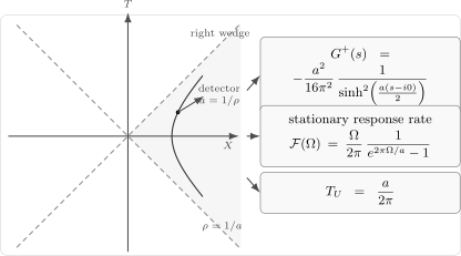
An eternally and uniformly accelerated detector samples a stationary KMS Wightman function with imaginary proper-time separation $2\pi/a$. Its long-time excitation rate is Planckian at $T_U=a/(2\pi)$; finite switching adds transients.

Nothing in this calculation says that the Minkowski vacuum is a thermal state for inertial observers. It says that the pair consisting of a state and a time evolution is thermal: the Minkowski vacuum, restricted to right-wedge observables, is thermal with respect to the boost generator.

Euclidean smoothness and the geometric temperature

There is a geometric way to see the same inverse temperature without calculating detector rates. Start from the right-wedge metric

$$ds^2=\rho^2d\eta^2-d\rho^2-d\mathbf y^2.$$

Continue to Euclidean boost time by setting

$$\eta=-i\theta.$$

and define the positive Euclidean line element by $ds_E^2=-ds^2$. Then

$$ds_E^2=d\rho^2+\rho^2d\theta^2+d\mathbf y^2.$$

The $(\rho,\theta)$ part is just the flat Euclidean plane in polar coordinates. The point $\rho=0$ is smooth only if

$$\theta\sim\theta+2\pi.$$

If an observer uses proper time $\tau=\eta/a$, then Euclidean proper time is $\tau_E=\theta/a$, and the period is

$$\tau_E\sim \tau_E+{2\pi\over a}.$$

Thermal QFT identifies Euclidean time period with inverse temperature, so again

$$\beta={2\pi\over a}, \qquad T_U={a\over2\pi}.$$

This argument is the flat-spacetime prototype of Hawking’s black-hole temperature calculation. Near any nonextremal horizon, the Euclidean metric looks like a plane in polar coordinates. Avoiding a conical singularity fixes the Euclidean period, and therefore fixes the temperature.

Wedge thermality and the regulated density-matrix picture

The detector calculation gives the operational meaning of the temperature. The operator-algebra statement is even sharper. Let $K_R$ be the dimensionless generator of Rindler time translations in the right wedge. With a UV regulator that factorizes left- and right-wedge degrees of freedom, one may write

$$\boxed{ \rho_R^{\rm(reg)} =\operatorname{Tr}_L |0_M\rangle\langle0_M| ={1\over Z_R}e^{-2\pi K_R}. }$$

Here $\operatorname{Tr}_L$ traces over degrees of freedom in the left wedge. If the physical Hamiltonian for proper time is

$$H_\tau=aK_R,$$

then

$$\rho_R^{\rm(reg)}={1\over Z_R}e^{-\beta H_\tau}, \qquad \beta={2\pi\over a}.$$

Mode by mode, the same regulated statement has the schematic thermofield-double form

$$|0_M\rangle \sim \prod_{\omega,\mathbf k} \left(1-e^{-2\pi\omega}\right)^{1/2} \sum_{n=0}^{\infty}e^{-\pi\omega n} |n_{\omega\mathbf k}\rangle_R|n_{\omega\mathbf k}\rangle_L.$$

Tracing over the left wedge gives

$$\rho_{R,\rm reg}^{(\omega,\mathbf k)} =\left(1-e^{-2\pi\omega}\right) \sum_{n=0}^{\infty}e^{-2\pi\omega n} |n_{\omega\mathbf k}\rangle_R\,{}_R\langle n_{\omega\mathbf k}|,$$

and hence

$$\langle N_{\omega\mathbf k}\rangle ={1\over e^{2\pi\omega}-1}.$$

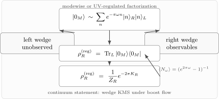
The global Minkowski vacuum is pure but entangled across the Rindler horizons. A modewise or UV-regulated factorization gives $\rho_R^{\rm(reg)}\propto e^{-2\pi K_R}$. Intrinsically, the continuum wedge state is KMS for boost flow rather than a trace-class density matrix.

The exact construction of the modes requires a careful choice of Unruh modes, but the thermal weights are fixed by analyticity and wedge localization. In continuum algebraic QFT, a wedge algebra is not generally represented by a tensor factor with a trace-class reduced density matrix; the literal partial trace above is a regulated mnemonic. The regulator-independent content is the KMS property of the vacuum under modular boost flow, as established by the Bisognano–Wichmann theorem under its standard axioms.

Summary

Thermal equilibrium can be characterized without mentioning particles: it is the KMS analyticity condition

$$\langle A(t)B(0)\rangle_\beta = \langle B(0)A(t+i\beta)\rangle_\beta.$$

In Fourier space, KMS becomes detailed balance. For a detector with level spacing $\Omega$,

$${\Gamma_\uparrow\over\Gamma_\downarrow}=e^{-\beta\Omega}.$$

In Euclidean field theory, the same condition becomes a compact imaginary-time circle of circumference $\beta$, with bosonic Matsubara frequencies $\omega_n=2\pi n/\beta$. Fluctuation–dissipation relates nonzero-frequency noise to the commutator spectrum; a conserved connected covariance gives an additional zero-frequency atom that the commutator does not determine.

For a uniformly accelerated observer, Rindler time is boost time. The Minkowski vacuum restricted to a single wedge is KMS with inverse temperature $2\pi$ in dimensionless boost time. Along a worldline of proper acceleration $a$, this becomes

$$\beta={2\pi\over a}, \qquad T_U={a\over2\pi}.$$

The Unruh effect is therefore not a statement that the inertial vacuum is globally mixed. It is a statement that the right-wedge restriction of the inertial vacuum is KMS with respect to boost evolution. The Planck formula is a stationary long-time detector rate; finite switching adds protocol-dependent transients. A reduced density matrix is a useful regulated or modewise representation, while the continuum theorem is intrinsically a statement about the wedge algebra and modular flow.

Common pitfalls

Replacing KMS by real-time periodicity. The shift is in imaginary time and, for real-time Wightman functions, changes operator ordering. The analytic strip and its boundary values are part of the statement.

Using the Feynman propagator to count detector clicks. Transition rates are controlled by the Wightman function evaluated along the detector trajectory, with the detector’s switching and $i0$ prescription specified.

Dividing by the KMS factor at zero frequency. A centered conserved observable can have nonzero thermal variance and zero commutator. Retain its $\delta(\omega)$ noise separately, and distinguish re-equilibration at fixed temperature from isolated dynamical response.

Calling the Minkowski vacuum a global thermal bath. The vacuum remains pure and Poincaré invariant. Thermality appears after restricting to one wedge and using boost evolution.

Forgetting which time generates the Hamiltonian. The inverse temperature is $2\pi$ for dimensionless boost time $\eta$. Along the trajectory $\eta=a\tau$, the proper inverse temperature is $2\pi/a$.

Treating a finite-time response as exactly Planckian. The compact response formula is a stationary long-time rate for uniform acceleration. A finite switching function produces transients that depend on the measurement protocol.

Confusing the Rindler and Minkowski vacua. The Rindler vacuum is empty for $K_R$ modes but singular at the horizons. The Minkowski vacuum is regular there and KMS when restricted to a wedge.

Taking the continuum partial trace literally. A UV regulator can supply a left–right tensor factor and a reduced density matrix. The intrinsic continuum statement is the KMS/modular-flow relation for the wedge algebra.

Exercises

Exercise 1: Derive KMS from trace cyclicity

Let

$$C^>_{AB}(t)=Z^{-1}\operatorname{Tr}\left(e^{-\beta H}A(t)B(0)\right).$$

Using $A(t-i\beta)=e^{\beta H}A(t)e^{-\beta H}$, prove

$$C^>_{AB}(t-i\beta)=C^<_{AB}(t), \qquad C^<_{AB}(t)=Z^{-1}\operatorname{Tr}\left(e^{-\beta H}B(0)A(t)\right).$$

Solution

Start from

$$C^>_{AB}(t-i\beta) ={1\over Z}\operatorname{Tr}\left(e^{-\beta H}A(t-i\beta)B(0)\right).$$

Substitute

$$A(t-i\beta)=e^{\beta H}A(t)e^{-\beta H}.$$

Then

$$C^>_{AB}(t-i\beta) ={1\over Z}\operatorname{Tr}\left(e^{-\beta H}e^{\beta H}A(t)e^{-\beta H}B(0)\right) ={1\over Z}\operatorname{Tr}\left(A(t)e^{-\beta H}B(0)\right).$$

By cyclicity of the trace,

$$\operatorname{Tr}\left(A(t)e^{-\beta H}B(0)\right) =\operatorname{Tr}\left(e^{-\beta H}B(0)A(t)\right).$$

Therefore

$$C^>_{AB}(t-i\beta)=C^<_{AB}(t).$$

Exercise 2: Detailed balance in frequency space

For a Hermitian operator $J$, define

$$G^>(t)=\langle J(t)J(0)\rangle_\beta, \qquad G^>(\omega)=\int dt\,e^{i\omega t}G^>(t).$$

Show that

$$G^>(-\omega)=e^{-\beta\omega}G^>(\omega).$$

Solution

Insert energy eigenstates:

$$G^>(t)={1\over Z}\sum_{m,n}e^{-\beta E_m}e^{i(E_m-E_n)t}|J_{mn}|^2.$$

Fourier transforming gives

$$G^>(\omega)={2\pi\over Z}\sum_{m,n}e^{-\beta E_m}|J_{mn}|^2 \delta\left(\omega-(E_n-E_m)\right).$$

Now compute $G^>(-\omega)$:

$$G^>(-\omega)={2\pi\over Z}\sum_{m,n}e^{-\beta E_m}|J_{mn}|^2 \delta\left(-\omega-(E_n-E_m)\right).$$

Relabel $m\leftrightarrow n$:

$$G^>(-\omega)={2\pi\over Z}\sum_{m,n}e^{-\beta E_n}|J_{mn}|^2 \delta\left(-\omega-(E_m-E_n)\right).$$

The delta function is now

$$\delta\left(\omega-(E_n-E_m)\right).$$

On its support,

$$E_n=E_m+\omega,$$

so

$$e^{-\beta E_n}=e^{-\beta\omega}e^{-\beta E_m}.$$

Therefore

$$G^>(-\omega)=e^{-\beta\omega}G^>(\omega).$$

Exercise 3: Matsubara frequencies from periodicity

Let $G_E(\tau)$ be a bosonic Euclidean thermal correlator satisfying

$$G_E(\tau+\beta)=G_E(\tau).$$

Show that its Fourier series contains only frequencies $\omega_n=2\pi n/\beta$. Then solve

$$\left(-{d^2\over d\tau^2}+\omega_0^2\right)G_E(\tau)=\delta_\beta(\tau)$$

in frequency space.

Solution

A periodic function on a circle of circumference $\beta$ has Fourier expansion

$$G_E(\tau)=\sum_{n\in\mathbb Z}c_n e^{i\omega_n\tau}.$$

The condition $G_E(\tau+\beta)=G_E(\tau)$ requires

$$e^{i\omega_n\beta}=1,$$

so

$$\omega_n={2\pi n\over\beta}.$$

Normalize the expansion as

$$G_E(\tau)={1\over\beta}\sum_{n\in\mathbb Z}G_n e^{i\omega_n\tau}, \qquad \delta_\beta(\tau)={1\over\beta}\sum_{n\in\mathbb Z}e^{i\omega_n\tau}.$$

Substitution into

$$\left(-{d^2\over d\tau^2}+\omega_0^2\right)G_E(\tau)=\delta_\beta(\tau)$$

gives

$$(\omega_n^2+\omega_0^2)G_n=1.$$

Hence

$$G_n={1\over\omega_n^2+\omega_0^2},$$

and

$$G_E(\tau)={1\over\beta}\sum_{n\in\mathbb Z} {e^{i\omega_n\tau}\over\omega_n^2+\omega_0^2}.$$

Exercise 4: Euclidean Rindler periodicity

Starting from

$$ds^2=\rho^2d\eta^2-d\rho^2,$$

set $\eta=-i\theta$ and show that smoothness at $\rho=0$ requires $\theta\sim\theta+2\pi$. Then derive the Unruh temperature for an observer whose proper time is $\tau=\eta/a$.

Solution

The continuation $\eta=-i\theta$, together with $ds_E^2=-ds^2$ for the mostly-minus convention, gives

$$ds_E^2=d\rho^2+\rho^2d\theta^2.$$

This is the Euclidean plane in polar coordinates. The point $\rho=0$ is smooth only if the angular coordinate has its standard period,

$$\theta\sim\theta+2\pi.$$

If $\eta=a\tau$, then after continuation $\theta=a\tau_E$. The period of Euclidean proper time is therefore

$$a\tau_E\sim a\tau_E+2\pi,$$

or

$$\tau_E\sim\tau_E+{2\pi\over a}.$$

Thermal field theory identifies the Euclidean time period with inverse temperature:

$$\beta={2\pi\over a}.$$

Thus

$$T_U={1\over\beta}={a\over2\pi}.$$

Exercise 5: Detailed balance for an accelerated detector

Assume the detector response function satisfies the KMS consequence

$$\mathcal F(\Omega)=e^{-\beta\Omega}\mathcal F(-\Omega)$$

for $\Omega>0$. Show that a two-level detector with energies $E_g=0$ and $E_e=\Omega$ relaxes to thermal occupation probabilities.

Solution

Let $p_g$ and $p_e$ be the probabilities for the ground and excited states. In equilibrium, the upward and downward probability currents balance:

$$p_g\Gamma_\uparrow=p_e\Gamma_\downarrow.$$

The rates are proportional to the response functions,

$$\Gamma_\uparrow\propto\mathcal F(\Omega), \qquad \Gamma_\downarrow\propto\mathcal F(-\Omega).$$

Using detailed balance,

$${\Gamma_\uparrow\over\Gamma_\downarrow} ={\mathcal F(\Omega)\over\mathcal F(-\Omega)} =e^{-\beta\Omega}.$$

Thus

$${p_e\over p_g}={\Gamma_\uparrow\over\Gamma_\downarrow}=e^{-\beta\Omega}.$$

This is exactly the thermal Boltzmann ratio for a two-level system:

$$p_g={1\over1+e^{-\beta\Omega}}, \qquad p_e={e^{-\beta\Omega}\over1+e^{-\beta\Omega}}.$$

For a uniformly accelerated detector in the Minkowski vacuum, $\beta=2\pi/a$.

Exercise 6: De-excitation from the stationary response

The stationary accelerated-detector response rate for a massless scalar in four dimensions can be written as

$$\mathcal F(\Omega)={\Omega\over2\pi}{1\over e^{2\pi\Omega/a}-1}.$$

Show that for $\Omega=-E<0$, with $E>0$, this becomes

$$\mathcal F(-E)={E\over2\pi}\left(1+{1\over e^{2\pi E/a}-1}\right).$$

Solution

Substitute $\Omega=-E$:

$$\mathcal F(-E)={-E\over2\pi}{1\over e^{-2\pi E/a}-1}.$$

Multiply numerator and denominator by $e^{2\pi E/a}$:

$$\mathcal F(-E)={E\over2\pi}{e^{2\pi E/a}\over e^{2\pi E/a}-1}.$$

Since

$${e^x\over e^x-1}=1+{1\over e^x-1},$$

we get

$$\mathcal F(-E)={E\over2\pi}\left(1+{1\over e^{2\pi E/a}-1}\right).$$

The $1$ is spontaneous emission; the Bose–Einstein term is stimulated emission.

Exercise 7: Noise that survives a vanishing commutator

Let $H=\Delta\sigma_z/2$ with $\Delta>0$, $J=\sigma_x+\kappa\sigma_z$ with real $\kappa$, and $r=\tanh(\beta\Delta/2)$. Find the connected symmetrized spectrum and commutator spectrum. Then compare the isothermal susceptibility for $H-fJ$ with the isolated retarded susceptibility at zero frequency.

Solution

The thermal mean is $\langle J\rangle=-\kappa r$. The $\sigma_x$ matrix elements connect the levels separated by $\Delta$, while $\kappa(\sigma_z+r)$ is conserved. Its variance is

$$C_0=\kappa^2(1-r^2).$$

Writing the lower and upper thermal probabilities as $p_-=(1+r)/2$ and $p_+=(1-r)/2$, the spectral sum gives

$$G_c^>(\omega)=2\pi\left[ p_-\delta(\omega-\Delta)+p_+\delta(\omega+\Delta) +C_0\delta(\omega)\right].$$

Consequently,

$$\begin{aligned} S_c(\omega)&=\pi\left[\delta(\omega-\Delta)+\delta(\omega+\Delta)\right] +2\pi C_0\delta(\omega),\\ \rho(\omega)&=2\pi r\left[\delta(\omega-\Delta)-\delta(\omega+\Delta)\right]. \end{aligned}$$

The nonzero-frequency noise is recovered from $\rho$ by the $\coth$ factor, but $C_0$ is absent from $\rho$. The imaginary-time connected correlator is

$$\langle\delta J(-i\lambda)\delta J(0)\rangle =p_-e^{-\lambda\Delta}+p_+e^{\lambda\Delta}+C_0.$$

Its integral yields

$$\chi_T={2r\over\Delta}+\beta C_0.$$

The commutator is $-2ir\sin(\Delta t)$, so the physical response kernel for $H-fJ$ is $\chi_R(t)=2r\theta(t)\sin(\Delta t)$. With an adiabatic factor $e^{-\epsilon t}$ and then $\epsilon\downarrow0$,

$$\chi_R(0)=\lim_{\epsilon\downarrow0} \int_0^\infty dt\,e^{-\epsilon t}2r\sin(\Delta t) ={2r\over\Delta}.$$

Thus $\chi_T-\chi_R(0)=\beta C_0$. The extra term comes from changing conserved-state probabilities during re-equilibration. Even at $\kappa=0$, the quantum result $2r/\Delta$ is generally different from $\beta\operatorname{Var}(\sigma_x)=\beta$.

References

• J. J. Bisognano and E. H. Wichmann, “On the Duality Condition for a Hermitian Scalar Field,” Journal of Mathematical Physics 16 (1975), 985–1007, doi:10.1063/1.522605.
• J. J. Bisognano and E. H. Wichmann, “On the Duality Condition for Quantum Fields,” Journal of Mathematical Physics 17 (1976), 303–321, doi:10.1063/1.522898.
• P. C. W. Davies, “Scalar Particle Production in Schwarzschild and Rindler Metrics,” Journal of Physics A: Mathematical and General 8 (1975), 609–616, doi:10.1088/0305-4470/8/4/022.
• S. A. Fulling, “Nonuniqueness of Canonical Field Quantization in Riemannian Space-Time,” Physical Review D 7 (1973), 2850–2862, doi:10.1103/PhysRevD.7.2850.
• R. Kubo, “Statistical-Mechanical Theory of Irreversible Processes. I. General Theory and Simple Applications to Magnetic and Conduction Problems,” Journal of the Physical Society of Japan 12 (1957), 570–586, doi:10.1143/JPSJ.12.570.
• P. C. Martin and J. Schwinger, “Theory of Many-Particle Systems. I,” Physical Review 115 (1959), 1342–1373, doi:10.1103/PhysRev.115.1342.
• W. G. Unruh, “Notes on Black-Hole Evaporation,” Physical Review D 14 (1976), 870–892, doi:10.1103/PhysRevD.14.870.

Further reading

• N. D. Birrell and P. C. W. Davies, Quantum Fields in Curved Space, Cambridge Monographs on Mathematical Physics, Cambridge University Press, Cambridge, 1982.
• R. Haag, Local Quantum Physics: Fields, Particles, Algebras, 2nd ed., Springer, Berlin, 1996.
• M. Le Bellac, Thermal Field Theory, Cambridge Monographs on Mathematical Physics, Cambridge University Press, Cambridge, 1996.
• S. Takagi, “Vacuum Noise and Stress Induced by Uniform Acceleration: Hawking–Unruh Effect in Rindler Manifold of Arbitrary Dimension,” Progress of Theoretical Physics Supplement 88 (1986), 1–142, doi:10.1143/PTPS.88.1.
• R. M. Wald, Quantum Field Theory in Curved Spacetime and Black Hole Thermodynamics, Chicago Lectures in Physics, University of Chicago Press, Chicago, 1994.