Schwinger–Dyson Identities and the Classical Limit

The previous page showed how perturbation theory can be generated by functional derivatives with respect to a source. This page extracts a deeper consequence of the same formalism: the path integral is invariant under changes of integration variables. An infinitesimal change of the field variable gives exact identities among correlation functions. These are the Schwinger–Dyson identities.

They are sometimes called the quantum equations of motion. Here that means an identity for a regulated path integral with specified boundary data and vanishing integration-by-parts boundary flux. An Euler–Lagrange insertion in that integral produces contact terms when it differentiates the other insertions. In the corresponding operator calculation, the same contacts arise when spacetime derivatives act outside time ordering and differentiate its step functions. Inserting a vanishing operator equation inside ordinary time ordering is a different operation.

This page also explains the classical expansion on a regular contributing saddle branch. With that assumption, the leading source-dependent expectation value obeys the classical sourced field equation, while connected quantum corrections are organized by powers of $\hbar$ and loop order. The exact Schwinger–Dyson identity alone does not establish this asymptotic regime.

This derivation uses source differentiation to insert fields and time-ordering contacts to differentiate an ordered correlator. The regulated Schwinger–Dyson construction supplies the finite integration problem behind the continuum notation used below.

Total derivatives in field space

Equation-of-motion sign and restored hbar

We use a real Lorentzian scalar field with

$$S[\phi]=\int d^dx\left[\frac12\partial_\mu\phi\partial^\mu\phi-\frac12m^2\phi^2-V(\phi)\right].$$

Thus

$$\frac{\delta S}{\delta\phi(x)}=-\left[(\Box+m^2)\phi(x)+V'(\phi(x))\right],$$

and the classical equation of motion is

$$(\Box+m^2)\phi+V'(\phi)=0.$$

We temporarily restore $\hbar$ in the section on the classical limit. Elsewhere, setting $\hbar=1$ recovers the course convention.

Begin with a normalized path-integral expectation value, denoted by a PI subscript:

$$\langle\mathcal O[\phi]\rangle_{\mathrm{PI}} =\frac{\int\mathcal D\phi\,\mathcal O[\phi]e^{iS[\phi]}} {\int\mathcal D\phi\,e^{iS[\phi]}}.$$

This notation abbreviates a fixed finite regulator, a compatible integration domain or contour, and the boundary prescription selecting the vacuum Feynman functional. Assume its zero-source denominator is nonzero. The action in a regulated identity includes the regulating terms; a regulated kinetic kernel and identity kernel replace $\Box+m^2$ and $\delta^{(d)}$ before the corresponding continuum limits are taken.

The field $\phi$ is an integration variable. A change of variables leaves an integral unchanged only when its domain and Jacobian are transformed as well. To obtain the zero on the next line, assume a flat regulated measure and vanishing boundary flux for the permitted variation: for example, an appropriate damped contour with sufficient endpoint falloff. Under these conditions,

$$0=\int\mathcal D\phi\, \frac{\delta}{\delta\phi(x)} \left[\mathcal O[\phi]e^{iS[\phi]}\right].$$

Expanding the derivative gives

$$0=\int\mathcal D\phi\,e^{iS[\phi]} \left[ \frac{\delta\mathcal O}{\delta\phi(x)} +i\mathcal O[\phi]\frac{\delta S}{\delta\phi(x)} \right].$$

After dividing by the vacuum functional, the basic Schwinger–Dyson identity is

$$\boxed{ \left\langle\mathcal O[\phi]\frac{\delta S}{\delta\phi(x)}\right\rangle_{\mathrm{PI}} =i\left\langle\frac{\delta\mathcal O}{\delta\phi(x)}\right\rangle_{\mathrm{PI}}. }$$

The identity is the field-theory analogue of the elementary integration-by-parts formula on a contour with vanishing endpoint term,

$$0=\int dq\,\frac{d}{dq}\left[f(q)e^{iS(q)}\right].$$

The sign in the boxed identity is worth checking once. From $0=\langle\delta\mathcal O/\delta\phi\rangle+i\langle\mathcal O\,\delta S/\delta\phi\rangle$, division by $i$ gives $\langle\mathcal O\,\delta S/\delta\phi\rangle=i\langle\delta\mathcal O/\delta\phi\rangle$, because $1/i=-i$. This small algebraic point prevents many wrong signs in contact-term formulas.

The boundary condition is consequential. On a finite interval with $S=0$ and $f(q)=q$, the same total derivative has integral $\int_0^a dq\,f'(q)=a$, not zero, although the local measure $dq$ is translation invariant. If its normalized field-space boundary term is $\mathcal B_{\mathcal O,x}$, the right-hand side of the boxed identity is instead $i\langle\delta\mathcal O/\delta\phi(x)\rangle_{\mathrm{PI}}-i\mathcal B_{\mathcal O,x}$. A nonflat measure contributes its logarithmic derivative as well.

Products at coincident spacetime points also need the regulator. Removing it requires defined renormalized composite insertions and their contact terms; the formal pointwise Euler–Lagrange polynomial does not supply that definition. A more general field redefinition can introduce a Jacobian contribution, which must be retained rather than inferred to vanish from the translation example.

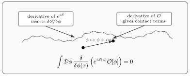
A Schwinger–Dyson identity is regulated integration by parts with vanishing boundary flux. Differentiating the exponential gives the path-integral equation-of-motion insertion; differentiating the other insertion gives contact terms. The field-space picture is schematic.

Contact terms from field insertions

Now choose the operator insertion to be a product of fields,

$$\mathcal O[\phi]=\phi(x_1)\phi(x_2)\cdots\phi(x_n).$$

Its functional derivative is

$$\frac{\delta\mathcal O}{\delta\phi(x)} =\sum_{j=1}^n\delta^{(d)}(x-x_j) \phi(x_1)\cdots\widehat{\phi(x_j)}\cdots\phi(x_n),$$

where the hat means that the factor is omitted. Let $G_n$ denote the full field moments generated by the same normalized vacuum functional; an empty product has expectation one. For field insertions without time derivatives, these are the usual vacuum time-ordered correlators in the compatible operator construction. Therefore

$$\boxed{ \left\langle\frac{\delta S}{\delta\phi(x)} \phi(x_1)\cdots\phi(x_n)\right\rangle_{\mathrm{PI}} =i\sum_{j=1}^n\delta^{(d)}(x-x_j) G_{n-1}(x_1,\ldots,\widehat{x_j},\ldots,x_n). }$$

The PI label is essential on this equation-of-motion insertion. It is not ordinary $\mathcal T$ applied to the operator $\delta S/\delta\widehat\phi$ after using an operator field equation. Some treatments encode this derivative prescription using a covariant $\mathcal T^\ast$ product; here the PI label keeps it explicit. The operator/path-integral distinction is explained by Schwartz 2014, § 14.7.2, p. 275.

Substituting the scalar action and taking the linear kinetic operator outside the field moment gives the Green-function equation

$$\boxed{ \begin{aligned} &(\Box_x+m^2)G_{n+1}(x,x_1,\ldots,x_n) +\left\langle\mathcal T V'(\phi(x))\phi(x_1)\cdots\phi(x_n)\right\rangle \\ &\qquad =-i\sum_{j=1}^n\delta^{(d)}(x-x_j) G_{n-1}(x_1,\ldots,\widehat{x_j},\ldots,x_n). \end{aligned} }$$

For a free scalar field, $V=0$, so

$$(\Box_x+m^2)G_{n+1}(x,x_1,\ldots,x_n) =-i\sum_{j=1}^n\delta^{(d)}(x-x_j) G_{n-1}(x_1,\ldots,\widehat{x_j},\ldots,x_n).$$

The two-point case is the familiar propagator equation

$$(\Box_x+m^2)D_F(x-y)=-i\delta^{(d)}(x-y).$$

Here $D_F=G_2$ in the free theory is the raw Feynman correlator; the delta-normalized inverse is $G_F=iD_F$. The operator $\Box_x+m^2$ acts on the whole ordered correlator. It annihilates it away from $x=y$ but differentiates ordering step functions at coincidence, producing the delta-function source. The direct operator derivation and interacting extension appear in Schwartz 2014, § 14.7.1, pp. 273–274.

The free oscillator makes the distinction explicit. For $P=\partial_t^2+\omega^2$ and $q(t)=(ae^{-i\omega t}+a^\dagger e^{i\omega t})/\sqrt{2\omega}$, the operator equation is $Pq=0$. Consequently,

$$\langle\mathcal T\{(Pq)(t)q(0)\}\rangle=0, \qquad P_t\langle\mathcal T\{q(t)q(0)\}\rangle=-i\delta(t).$$

Indeed $D(t)=e^{-i\omega|t|}/(2\omega)$ is continuous, while $D'(0^+)-D'(0^-)=-i$. That derivative jump supplies the delta function. See coincident products and contact terms for the corresponding field calculation.

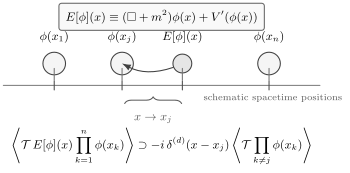
In the regulated path-integral identity, $E[\phi]=(\Box+m^2)\phi+V'(\phi)$ has a contact with negative coefficient $-i$ when the variation reaches $\phi(x_j)$. The PI bracket denotes that insertion prescription, not ordinary time ordering of a vanishing operator equation. The locations are schematic; delta functions denote distributional contacts, not finite regions around the drawn points.

For an interacting theory, the same equation becomes a hierarchy. If

$$V(\phi)=\frac{\lambda}{4!}\phi^4,$$

then

$$V'(\phi)=\frac{\lambda}{3!}\phi^3,$$

and the two-point equation, exact at the fixed compatible regulator, is

$$\boxed{ (\Box_x+m^2)G_2(x,y) +\frac{\lambda}{3!}\langle\mathcal T\phi^3(x)\phi(y)\rangle =-i\delta^{(d)}(x-y). }$$

Here $\phi^3(x)$ abbreviates the regulated coincident insertion in a theory with a nonderivative potential. A continuum renormalized identity needs the renormalized composite operator, any mixing, and the corresponding contact prescription. The two-point function is therefore coupled to a four-field expectation value. Applying the identity to that four-field expectation value produces six-field expectations, and so on. The hierarchy is exact at the regulated level but infinite. Perturbation theory solves it order by order by evaluating the higher correlators with Wick contractions. Conceptually, this is the quantum version of a nonlinear equation: the equation for an average field or two-point function does not close because fluctuations of all orders feed back into it.

Source-functional form

The same identity can be packed into one functional differential equation. Define the unnormalized source functional

$$Z[J]=\int\mathcal D\phi\, \exp\left(iS[\phi]+i\int d^dx\,J(x)\phi(x)\right).$$

The total derivative with no extra insertion gives

$$0=\int\mathcal D\phi\, \left(\frac{\delta S}{\delta\phi(x)}+J(x)\right) \exp\left(iS[\phi]+i\int J\phi\right).$$

Inside $Z[J]$, multiplication by $\phi(x)$ is represented by

$$\phi(x)\longleftrightarrow \frac1i\frac{\delta}{\delta J(x)}.$$

Thus

$$\boxed{ \left[ \frac{\delta S}{\delta\phi(x)}\bigg|_{\phi\to (1/i)\delta/\delta J} +J(x) \right]Z[J]=0. }$$

For the scalar action above this becomes

$$\boxed{ \left[ (\Box_x+m^2)\frac1i\frac{\delta}{\delta J(x)} +V'\left(\frac1i\frac{\delta}{\delta J(x)}\right) -J(x) \right]Z[J]=0. }$$

The minus sign in front of $J$ is a consequence of the action convention $\delta S/\delta\phi=-[(\Box+m^2)\phi+V'(\phi)]$. If one writes the Schwinger–Dyson equation directly in terms of $\delta S/\delta\phi+J$, the same statement appears with the opposite overall sign. Multiplying the whole functional equation by $-1$ changes nothing, but changing only the $J$ sign would be wrong.

For $\lambda\phi^4/4!$ theory,

$$\left[ (\Box_x+m^2)\frac1i\frac{\delta}{\delta J(x)} +\frac{\lambda}{3!}\left(\frac1i\frac{\delta}{\delta J(x)}\right)^3 -J(x) \right]Z[J]=0.$$

Taking derivatives of this equation with respect to $J$ and then setting $J=0$ reproduces the whole regulated Schwinger–Dyson hierarchy. In the compatible operator construction, the kinetic operator acts outside time ordering; derivatives of its step functions give the same contacts. It must not be moved through $\mathcal T$ and replaced by an already vanishing free operator equation.

The tadpole from the Schwinger–Dyson equation

The first-order tadpole correction to the two-point function can be derived directly from the exact identity. Write

$$G_2(x,y)=G_0(x,y)+G_2^{(1)}(x,y)+O(\lambda^2),$$

where $G_2^{(1)}$ is the order-$\lambda$ correction to the two-point function. This notation keeps it distinct from the one-point function $G_1(x)$. The free propagator satisfies

$$(\Box_x+m^2)G_0(x,y)=-i\delta^{(d)}(x-y).$$

The order-$\lambda$ part of the two-point Schwinger–Dyson equation is

$$(\Box_x+m^2)G_2^{(1)}(x,y) =-\frac{\lambda}{3!}\langle\mathcal T\phi^3(x)\phi(y)\rangle_0.$$

By Wick theorem,

$$\langle\mathcal T\phi^3(x)\phi(y)\rangle_0 =3G_0(x,x)G_0(x,y).$$

Thus

$$(\Box_x+m^2)G_2^{(1)}(x,y) =-\frac{\lambda}{2}G_0(x,x)G_0(x,y).$$

Since $(\Box_x+m^2)G_0(x,z)=-i\delta^{(d)}(x-z)$, the inverse of $\Box+m^2$ with Feynman boundary conditions is $iG_0$. Therefore

$$\boxed{ G_2^{(1)}(x,y) =-\frac{i\lambda}{2}\int d^dz\, G_0(x,z)G_0(z,z)G_0(z,y). }$$

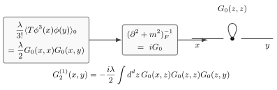
The Schwinger–Dyson equation turns the interaction term $\lambda\phi^3/3!$ into the free contraction $3G_0(x,x)G_0(x,y)$. Inverting the free Klein–Gordon operator attaches another propagator and gives the tadpole correction to $G_2$.

The coincident propagator $G_0(z,z)$ is the important warning sign. In continuum field theory it is generally ultraviolet divergent. The local divergence has the form of a correction to the mass term, which is why tadpoles become part of mass renormalization.

Classical limit from stationary phase

Now restore $\hbar$:

$$Z[J]=\int\mathcal D\phi\, \exp\left[\frac{i}{\hbar}\left(S[\phi]+\int d^dx\,J\phi\right)\right].$$

The source-functional Schwinger–Dyson equation becomes

$$\boxed{ \left[ \frac{\delta S}{\delta\phi(x)}\bigg|_{\phi\to (\hbar/i)\delta/\delta J} +J(x) \right]Z[J]=0. }$$

For the classical expansion, keep a finite regulator $R$ and use real integration coordinates, a smooth real action, and $\hbar$-independent couplings and sources. Assume that a contributing isolated saddle of $S+\int J\phi$ varies smoothly in a small source neighborhood and has a nonsingular Hessian there. Use the continued Lorentzian Gaussian prescription of the stationary-phase calculation: remove its damping at fixed $R$ and $\hbar$ before taking $\hbar\to0$. Negative Hessian eigenvalues change Gaussian phases; they do not by themselves invalidate the expansion.

To approximate the full $Z[J]$ by this branch, require the other saddle, endpoint, and complementary contributions to be subleading, also after the source derivatives used below. Assume $Z[J]\ne0$ in this neighborhood, so a local $W=-i\hbar\log Z$ exists, and that its source-dependent part has a differentiable asymptotic expansion with bounded source derivatives. A smooth local cutoff can isolate a saddle for asymptotic analysis, but the exact Schwinger–Dyson identity still uses the original integration domain: inserting a cutoff adds its derivative term. Competing saddles, zeros of $Z$, and coalescing saddles require separate treatment, as does removal of $R$; see the regulated saddle expansion.

On this branch let

$$Z[J]=e^{iW[J]/\hbar}, \qquad \varphi_J(x)=\frac{\delta W[J]}{\delta J(x)}.$$

The field $\varphi_J$ is the source-dependent expectation value of $\phi$. Since

$$\frac{\hbar}{i}\frac{\delta Z}{\delta J(x)}=\varphi_J(x)Z[J],$$

successive derivatives separate products of mean fields from connected fluctuations. With finite source indices and $D_a=(\hbar/i)\partial_{J_a}$, the exact identity is

$$\frac{D_aD_b Z}{Z} =\varphi_{J,a}\varphi_{J,b} +\frac{\hbar}{i}\,\partial_{J_a}\varphi_{J,b}.$$

The last term is suppressed only if the source derivative stays bounded. Write $\varphi_J=\varphi_{0,J}+O(\hbar)$ for the assumed regular expansion. Repeated differentiation then gives the leading equation

$$\boxed{ \left.\frac{\delta S}{\delta\phi(x)}\right|_{\phi=\varphi_{0,J}}+J(x)=0. }$$

With the action convention of this page,

$$(\Box+m^2)\varphi_{0,J}(x)+V'(\varphi_{0,J}(x))=J(x).$$

This equation is for the leading field, not the exact quantum mean. It can be nonlinear and interacting. Let $H_{ab}$ be the finite-regulator action Hessian evaluated at $\varphi_{0,J}$. Differentiating the saddle equation gives $H_{ab}\partial_{J_c}\varphi_{0,J,b}=-\delta_{ac}$, so $\partial_{J_c}\varphi_{0,J,b}=-(H^{-1})_{bc}$. A uniformly nonsingular Hessian on a compact source neighborhood gives a bounded leading response.

The same result follows from stationary phase. Define the source-dependent phase functional

$$S_J[\phi] =S[\phi]+\int d^dx\,J(x)\phi(x),$$

and expand around the chosen saddle $\phi_{\mathrm{cl},J}=\varphi_{0,J}$:

$$\phi(x)=\phi_{\mathrm{cl},J}(x)+\sqrt{\hbar}\,\eta(x), \qquad \left.\frac{\delta S_J}{\delta\phi(x)} \right|_{\phi=\phi_{\mathrm{cl},J}}=0.$$

At fixed $R$ and bounded fluctuation coordinates, Taylor expansion gives

$$S_J[\phi_{\mathrm{cl},J}+\sqrt{\hbar}\eta] =S_J[\phi_{\mathrm{cl},J}] +\frac{\hbar}{2}\int d^dx\,d^dy\,\eta(x)S^{(2)}(x,y)\eta(y) +O(\hbar^{3/2}).$$

The linear term vanishes by the sourced equation. The source is linear in $\phi$, so the Hessian is still $S^{(2)}$, evaluated on $\phi_{\mathrm{cl},J}$. Its continued Gaussian gives the local fluctuation determinant. The Taylor remainder above is not a uniform continuum estimate.

A degree-$n$ fluctuation vertex in $iS_J/\hbar$ carries $\hbar^{n/2-1}$. A connected vacuum graph with $I$ internal lines and $V$ vertices therefore carries $\hbar^{I-V}=\hbar^{L-1}$ in $\log Z$, where $L=I-V+1$ is its loop number. Since $W=-i\hbar\log Z$, its contribution is of order $\hbar^L$ in $W$. The classical term is tree level and the Gaussian determinant is one loop. This counting applies to the regular connected expansion and its source derivatives; source-independent normalization terms in $W$ need not form a pure power series.

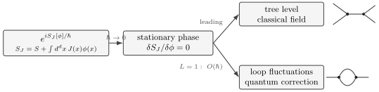
For the regular contributing branch described above, the classical sourced action leads $W[J]$; its connected loop corrections carry successive powers of $\hbar$. The diagram is schematic and does not assert dominance of every stationary configuration or uniform control when the regulator is removed.

Connected functions and the quantum equation of motion

The connected generator $W[J]$ makes the fluctuations explicit. In $\lambda\phi^4/4!$ theory, the exact regulated source equation decomposes into raw connected moments as

$$(\Box+m^2)\varphi_J(x) +\frac{\lambda}{3!}\left[ \varphi_J^3(x)+3\varphi_J(x)G_{J,c}(x,x)+G_{J,c}^{(3)}(x,x,x) \right] =J(x),$$

Here $\langle\cdot\rangle_J$ is the normalized regulated PI bracket with source $J$. For $\delta\phi=\phi-\varphi_J$, the raw cumulants are $G_{J,c}(x,y)=\langle\delta\phi(x)\delta\phi(y)\rangle_J$ and $G_{J,c}^{(3)}(x,y,z)=\langle\delta\phi(x)\delta\phi(y)\delta\phi(z)\rangle_J$. Thus

$$\begin{aligned} G_{J,c}(x,y) &=\frac{\hbar}{i}\frac{\delta^2W}{\delta J(x)\delta J(y)},\\ G_{J,c}^{(3)}(x,y,z) &=\left(\frac{\hbar}{i}\right)^2 \frac{\delta^3W}{\delta J(x)\delta J(y)\delta J(z)}. \end{aligned}$$

These identities are exact before taking coincident arguments at the common regulator. The orders $G_{J,c}=O(\hbar)$ and $G_{J,c}^{(3)}=O(\hbar^2)$ additionally use bounded source derivatives on the regular branch. The coincident terms are not undefined products of continuum distributions: removing the regulator requires renormalized composite insertions and the corresponding contact prescription.

Later this idea is sharpened using the effective action $\Gamma[\varphi]$, the Legendre transform of $W[J]$. Its equation of motion is

$$\frac{\delta\Gamma[\varphi]}{\delta\varphi(x)}=-J(x).$$

On a locally invertible source-to-field branch, its leading Legendre transform is $\Gamma_0=S$. Loop corrections give the quantum effective action; the exact Schwinger–Dyson identities continue to constrain it without assuming that every solution admits this expansion.

Related nonperturbative treatment

This lesson gives a first Lorentzian derivation, including contact terms, the tadpole, and the classical limit. Schwinger–Dyson Hierarchies and Renormalization Inputs continues to renormalized propagator and vertex hierarchies, closure choices, solution branches, and continuum methods.

Summary

Schwinger–Dyson identities follow from a permitted change of variables in a regulated path integral, with its measure, contour, and boundary terms accounted for. When the integration-by-parts flux vanishes, the PI insertion of $\delta S/\delta\phi$ is equivalent to differentiating the other insertions. For products of fields, these derivatives give contact terms supported at coincident points.

For a free scalar, the identity says that the Feynman propagator is a Green function of $\Box+m^2$. For an interacting scalar, it generates an infinite hierarchy: the two-point function is coupled to higher correlators through $V'(\phi)$. Perturbation theory solves this hierarchy order by order, and the first nontrivial example is the tadpole correction in $\phi^4$ theory.

On the stated regular contributing branch, the leading field $\varphi_{0,J}$ obeys the classical sourced equation, while connected fluctuations and loop corrections to $W$ have the derived powers of $\hbar$. The exact identity itself remains valid outside this particular asymptotic regime.

Common pitfalls

Do not identify $\langle\mathcal T\{(P\widehat\phi)\widehat\phi\}\rangle$ with $P\langle\mathcal T\{\widehat\phi\widehat\phi\}\rangle$. For a free field the first is zero; the second contains the contact from differentiating the ordering step functions.

Do not treat the Schwinger–Dyson identity as a perturbative statement. The identity is exact for its stated regulated integral and boundary conditions; perturbation theory is one method for approximately solving it.

Do not forget the sign of $\delta S/\delta\phi$. With the convention used here, $\delta S/\delta\phi=-[(\Box+m^2)\phi+V'(\phi)]$.

Do not assume that coincident quantities such as $G_0(x,x)$ are finite. They are usually ultraviolet divergent and must be regulated.

Do not confuse a regular classical expansion with the free theory. Its leading field equation can be nonlinear. Small explicit powers of $\hbar$ do not suppress a term whose source derivatives become singular.

Exercises

Exercise 1

Under the stated vanishing-flux assumption, derive the regulated path-integral identity

$$\left\langle\frac{\delta S}{\delta\phi(x)} \phi(x_1)\cdots\phi(x_n)\right\rangle_{\mathrm{PI}} =i\sum_{j=1}^n\delta^{(d)}(x-x_j) G_{n-1}(x_1,\ldots,\widehat{x_j},\ldots,x_n).$$

Solution

Start from

$$0=\int\mathcal D\phi\, \frac{\delta}{\delta\phi(x)} \left[\phi(x_1)\cdots\phi(x_n)e^{iS[\phi]}\right].$$

Expanding the derivative gives

$$0=\int\mathcal D\phi\,e^{iS[\phi]} \left[ \sum_{j=1}^n\delta^{(d)}(x-x_j) \phi(x_1)\cdots\widehat{\phi(x_j)}\cdots\phi(x_n) +i\frac{\delta S}{\delta\phi(x)}\phi(x_1)\cdots\phi(x_n) \right].$$

Divide by the vacuum functional and rearrange:

$$\left\langle\frac{\delta S}{\delta\phi(x)} \phi(x_1)\cdots\phi(x_n)\right\rangle_{\mathrm{PI}} =i\sum_{j=1}^n\delta^{(d)}(x-x_j) G_{n-1}(x_1,\ldots,\widehat{x_j},\ldots,x_n).$$

Exercise 2

Use Wick theorem to verify the free identity

$$(\Box_x+m^2)G_4(x,x_1,x_2,x_3) =-i\sum_{j=1}^3\delta^{(d)}(x-x_j) G_2(x_1,\ldots,\widehat{x_j},\ldots,x_3).$$

Solution

For a free real scalar field,

$$\begin{aligned} G_4(x,x_1,x_2,x_3) &=G_0(x,x_1)G_0(x_2,x_3) +G_0(x,x_2)G_0(x_1,x_3)\\ &\quad+G_0(x,x_3)G_0(x_1,x_2). \end{aligned}$$

Acting with $\Box_x+m^2$ only affects the propagator containing $x$. Since

$$(\Box_x+m^2)G_0(x,x_j)=-i\delta^{(d)}(x-x_j),$$

we obtain

$$\begin{aligned} (\Box_x+m^2)G_4 &=-i\delta^{(d)}(x-x_1)G_0(x_2,x_3)\\ &\quad -i\delta^{(d)}(x-x_2)G_0(x_1,x_3)\\ &\quad -i\delta^{(d)}(x-x_3)G_0(x_1,x_2), \end{aligned}$$

which is the desired contact-term identity.

Exercise 3

For $V(\phi)=\lambda\phi^4/4!$, derive

$$G_2^{(1)}(x,y)=-\frac{i\lambda}{2}\int d^dz\,G_0(x,z)G_0(z,z)G_0(z,y)$$

from the two-point Schwinger–Dyson equation.

Solution

The exact two-point equation is

$$(\Box_x+m^2)G_2(x,y) +\frac{\lambda}{3!}\langle\mathcal T\phi^3(x)\phi(y)\rangle =-i\delta^{(d)}(x-y).$$

Set $G_2=G_0+G_2^{(1)}+O(\lambda^2)$. The free part satisfies

$$(\Box_x+m^2)G_0(x,y)=-i\delta^{(d)}(x-y).$$

At order $\lambda$,

$$(\Box_x+m^2)G_2^{(1)}(x,y) =-\frac{\lambda}{3!}\langle\mathcal T\phi^3(x)\phi(y)\rangle_0.$$

Wick theorem gives

$$\langle\mathcal T\phi^3(x)\phi(y)\rangle_0 =3G_0(x,x)G_0(x,y).$$

Therefore

$$(\Box_x+m^2)G_2^{(1)}(x,y) =-\frac{\lambda}{2}G_0(x,x)G_0(x,y).$$

Using the inverse relation $(\Box_x+m^2)G_0(x,z)=-i\delta^{(d)}(x-z)$ gives

$$G_2^{(1)}(x,y)=-\frac{i\lambda}{2}\int d^dz\,G_0(x,z)G_0(z,z)G_0(z,y).$$

Exercise 4

Use the regular contributing-branch assumptions of the classical-limit section, including bounded source derivatives and $Z[J]\ne0$. Restore $\hbar$, set $\varphi_J=\delta W/\delta J=\varphi_{0,J}+O(\hbar)$ with $Z=e^{iW/\hbar}$, and show that the leading field satisfies

$$\left.\frac{\delta S}{\delta\phi(x)}\right|_{\phi=\varphi_{0,J}}+J(x)=0.$$

Solution

With $\hbar$ restored,

$$\left[ \frac{\delta S}{\delta\phi(x)}\bigg|_{\phi\to (\hbar/i)\delta/\delta J} +J(x) \right]Z[J]=0.$$

Because $Z=e^{iW/\hbar}$,

$$\frac{\hbar}{i}\frac{\delta Z}{\delta J(x)} =\frac{\delta W}{\delta J(x)}Z =\varphi_J(x)Z.$$

Divide the exact identity by $Z[J]$. When several source derivatives act on $Z$, their product term uses $\varphi_J$; every term differentiating $\varphi_J$ has an explicit power of $\hbar$. The assumed bounded derivatives make those terms subleading. Substituting $\varphi_J=\varphi_{0,J}+O(\hbar)$ therefore gives

$$\frac{\delta S}{\delta\phi(x)}\bigg|_{\phi=\varphi_{0,J}}+J(x) =O(\hbar).$$

Taking the leading coefficient yields

$$\left.\frac{\delta S}{\delta\phi(x)}\right|_{\phi=\varphi_{0,J}}+J(x)=0.$$

Exercise 5

Use the free oscillator to distinguish an equation-of-motion insertion inside ordinary time ordering from a differential operator acting outside it. Explain which operation the path-integral identity represents, and what changes for interacting coincident products.

Solution

The free operator satisfies $(\partial_t^2+\omega^2)q(t)=0$, so ordinary time ordering of that zero operator with $q(0)$ is zero. Its ordered correlator is instead $D(t)=e^{-i\omega|t|}/(2\omega)$. The derivative jump is

$$D'(0^+)-D'(0^-) =-\frac{i}{2}-\frac{i}{2}=-i,$$

and therefore $(\partial_t^2+\omega^2)D=-i\delta$. The path-integral identity represents the latter differentiation prescription; since $\delta S/\delta q=-Pq$, its equation-of-motion insertion has the opposite contact sign. In field notation,

$$\left\langle\frac{\delta S}{\delta\phi(x)} \phi(x_1)\cdots\phi(x_n)\right\rangle_{\mathrm{PI}} =i\sum_{j=1}^n\delta^{(d)}(x-x_j) G_{n-1}(x_1,\ldots,\widehat{x_j},\ldots,x_n).$$

The right-hand side vanishes away from coincidence, but its contacts cannot be discarded in an integrated identity. For an interacting theory, $V'(\phi(x))$ is first a regulated composite insertion; its continuum counterpart requires renormalization and possible mixing. Neither a pointwise continuum product nor an interchange of differentiation and ordinary time ordering follows from the path-integral formula.

References

• Schwartz, Matthew D. Quantum Field Theory and the Standard Model. Cambridge University Press, 2014, § 14.7, pp. 273–275. Publisher DOI.

Further reading

• Mark Srednicki, Quantum Field Theory, Sections 9 and 22, for path integrals, source functionals, and Schwinger–Dyson equations.
• Sidney Coleman, Lectures of Sidney Coleman on Quantum Field Theory, Chapters 4, 7–8, and 28, for equations of motion, Dyson expansion, Wick diagrams, and functional integration.
• Steven Weinberg, The Quantum Theory of Fields, Volume I, Chapters 7 and 9, for canonical equations, path-integral methods, and source-functional reasoning.
• A. Zee, Quantum Field Theory in a Nutshell, Appendix A and Chapter I.12, for Gaussian identities and diagrammatic intuition from source functionals.