Symmetry Restoration and Mermin–Wagner Physics

The nonlinear sigma model looks, at first sight, like the perfect theory of an ordered magnet. Its field is a unit vector,

$$\mathbf n(x)^2=1,$$

and the action penalizes gradients, so the classical ground states are constant maps. A classical field can simply choose a direction on $S^{N-1}$. Quantum mechanically, and also statistically, that sentence is dangerous. In finite volume the path integral integrates over all directions. In low enough dimension, even an arbitrarily large system cannot hold a direction fixed, because the massless angular fluctuations are too strong in the infrared.

This page makes that statement quantitative. We use the $O(N)$ nonlinear sigma model to see three related facts: finite-volume symmetry restoration, the Mermin–Wagner infrared divergence, and the large-$N$ phase structure in general dimension. The same formulas also explain why two dimensions are special, why one-dimensional antiferromagnets have no conventional Néel order, and, for $N>2$, why the $2+\epsilon$ sigma-model expansion and the $4-\epsilon$ Landau–Ginzburg expansion describe the same critical universality class from opposite ends.

Required background. Nonlinear sigma models and constraints supplies the constrained-field action, and the large-$N$ saddle supplies the gap equation used below.

Helpful background. The sigma-model beta function explains the two-dimensional running coupling, while spin chains and theta terms motivates the final application.

Symmetry restoration in finite volume

Normalization for this page. We use the Euclidean $d$-dimensional $O(N)$ nonlinear sigma model

$$S[\mathbf n] ={1\over2\alpha_0}\int d^dx\,\partial_\mu\mathbf n\cdot\partial_\mu\mathbf n, \qquad \mathbf n^2=1.$$

The coupling $\alpha_0$ plays the role of a temperature or quantum fluctuation strength. Small $\alpha_0$ means a stiff, classically ordered field; large $\alpha_0$ means strong fluctuations.

For the large-$N$ discussion we enforce the constraint with a Lagrange multiplier,

$$S[\mathbf n,\lambda] ={1\over2\alpha_0}\int d^dx\, \left[(\partial_\mu\mathbf n)^2+\lambda(\mathbf n^2-1)\right].$$

At a constant saddle $\lambda=m^2$, the leading large-$N$ propagator is

$$\langle n^a(k)n^b(-k)\rangle ={\alpha_0\delta^{ab}\over k^2+m^2},$$

and the saddle condition is

$$N\alpha_0\int^\Lambda {d^dk\over(2\pi)^d}\,{1\over k^2+m^2}=1.$$

This is the same large-$N$ normalization as the previous sigma-model pages after setting $g_0=N\alpha_0$.

The action is invariant under

$$\mathbf n(x)\mapsto R\mathbf n(x), \qquad R\in O(N).$$

Therefore, in a finite box with no external field and with symmetry-preserving boundary conditions and regulator, the path integral cannot produce a vector expectation value:

$$\langle \mathbf n(x)\rangle=0.$$

This statement is not yet the Mermin–Wagner theorem. It is simpler: the path integral averages over the global zero mode. If a configuration with constant order parameter $\mathbf n_0$ contributes, then the rotated configuration $R\mathbf n_0$ contributes with the same weight. Averaging over all $R$ gives zero. A fixed boundary spin would already select a direction, so it belongs on the same footing as an external source rather than in the symmetric finite-volume ensemble.

The usual language of spontaneous symmetry breaking uses a particular order of limits. Choose a unit vector $\widehat{\mathbf h}$, add a small external field $\mathbf h=h\widehat{\mathbf h}$ with $h>0$,

$$S_h=S-\int d^dx\,\mathbf h\cdot\mathbf n(x),$$

and define the magnetization along the selected direction by

$$M = \lim_{h\to0^+}\lim_{V\to\infty} {1\over V}\int d^dx\, \widehat{\mathbf h}\cdot\langle\mathbf n(x)\rangle_{h\widehat{\mathbf h}}, \qquad \mathbf M=M\widehat{\mathbf h}.$$

The thermodynamic limit must come first. If one takes $\mathbf h\to0$ at fixed volume, symmetry is restored by the zero-mode integral and $\mathbf M=0$. If one first takes $V\to\infty$, the factor $V\mathbf h\cdot\mathbf n_0$ can become arbitrarily large even for tiny $\mathbf h$, and the path integral may localize near a chosen direction. That chosen direction is what one calls a pure broken-symmetry phase.

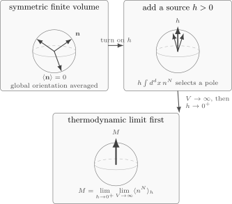
With symmetry-preserving finite-volume boundary conditions, the global orientation of the order parameter is integrated over and $\langle\mathbf n\rangle=0$. A small source $\mathbf h$ selects a direction. A nonzero order parameter is possible only when $V\to\infty$ is taken before $\mathbf h\to0$.

Thus the honest question is not whether a finite-volume path integral has $\langle\mathbf n\rangle\ne0$. It does not. The real question is whether the thermodynamic limit supports pure phases with a stable direction. The answer depends on the infrared behavior of the would-be Goldstone modes.

Two different restorations

There are two mechanisms in this page, and they should not be merged.

• Finite-volume restoration: with symmetric boundary conditions, the global zero mode is integrated over, so $\langle\mathbf n\rangle=0$ unless a source or boundary condition selects a direction.
• Infrared restoration: in $d\le2$, massless angular fluctuations diverge so strongly that even the thermodynamic limit cannot sustain a fixed continuous direction.

The first mechanism is kinematic and happens in any symmetric finite box. The second is dynamical and is the content of Mermin–Wagner/Coleman physics.

Spin waves and the infrared test

Suppose the system tries to order in the first internal direction. Locally write

$$\mathbf n=(\sigma,\boldsymbol\pi), \qquad \sigma=\sqrt{1-\boldsymbol\pi^2}, \qquad \boldsymbol\pi=(\pi^1,\ldots,\pi^{N-1}).$$

For small transverse fluctuations,

$$\sigma=1-{1\over2}\boldsymbol\pi^2+O(\pi^4),$$

and

$$\partial_\mu\mathbf n\cdot\partial_\mu\mathbf n =(\partial_\mu\boldsymbol\pi)^2+O(\pi^2(\partial\pi)^2).$$

The leading spin-wave action is therefore

$$S_{\rm sw} ={1\over2\alpha_0}\int d^dx\,(\partial_\mu\boldsymbol\pi)^2.$$

The transverse fields are massless Goldstone modes. Their propagator is

$$\langle\pi^i(k)\pi^j(-k)\rangle ={\alpha_0\delta^{ij}\over k^2}.$$

The fluctuation of the order-parameter direction is

$$\langle\boldsymbol\pi^2\rangle =(N-1)\alpha_0 \int_{1/L}^{\Lambda}{d^dk\over(2\pi)^d}\,{1\over k^2},$$

where $L$ is the box size and $\Lambda$ is the ultraviolet cutoff. The ultraviolet part depends on microscopic physics, but the infrared part decides whether long-range order is possible.

Writing $d^dk=S_{d-1}k^{d-1}dk$, where

$$S_{d-1}={2\pi^{d/2}\over\Gamma(d/2)},$$

we get

$$\int_{1/L}^{\Lambda}{d^dk\over(2\pi)^d}\,{1\over k^2} ={S_{d-1}\over(2\pi)^d} \int_{1/L}^{\Lambda}dk\,k^{d-3}.$$

Therefore

$$\int_{1/L}^{\Lambda}{d^dk\over(2\pi)^d}\,{1\over k^2} \sim \begin{cases} \displaystyle {S_{d-1}\over(2\pi)^d}{L^{2-d}\over 2-d}, & d<2,\\ \displaystyle {1\over2\pi}\log(\Lambda L), & d=2,\\ \displaystyle \text{finite as }L\to\infty, & d>2. \end{cases}$$

For $d\le2$, the transverse fluctuations diverge in the thermodynamic limit. The expansion around a fixed direction destroys itself: the would-be order parameter is washed out by arbitrarily long-wavelength angular modes. This is the spin-wave form of the Mermin–Wagner–Hohenberg mechanism for a $d$-dimensional equilibrium system, and of Coleman’s result when $d=2$ is interpreted as one space and one Euclidean-time dimension.

The divergence should be interpreted as a failure of the assumed ordered saddle, not as a literal statement that the microscopic field has infinite length. The constraint $\mathbf n^2=1$ remains exact. What diverges is the perturbative angular variance around any chosen direction.

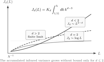
The stability of a continuous order parameter is tested by the Goldstone variance $(N-1)\alpha_0\int d^dk/k^2$. The infrared end of the integral diverges for $d\le2$, so a fixed direction cannot survive in the thermodynamic limit.

A useful way to phrase the same point is to estimate the magnetization in the ordered patch:

$$\langle n^1\rangle =\left\langle\sqrt{1-\boldsymbol\pi^2}\right\rangle \approx 1-{1\over2}\langle\boldsymbol\pi^2\rangle.$$

If $\langle\boldsymbol\pi^2\rangle$ diverges with $L$, the perturbative magnetization is not merely reduced; the assumption of a nonzero magnetization is inconsistent.

This argument applies to continuous internal symmetries in equilibrium systems with sufficiently short-range interactions and the usual regularity assumptions. Long-range forces, nonequilibrium steady states, gauge redundancies, and spacetime symmetries require separate analyses. It does not forbid phase transitions with discrete symmetry: the two-dimensional Ising model has a $\mathbb Z_2$ symmetry rather than a continuous sphere of broken directions. It also does not forbid topological transitions. The two-dimensional $O(2)$ model has no conventional magnetization, but its vortex physics leads to the Berezinskii–Kosterlitz–Thouless transition.

The O(2) check: algebraic order without magnetization

The $O(2)$ model is a clean check because the unit vector can be written as

$$\mathbf n=(\cos\theta,\sin\theta).$$

In a patch where $\theta$ is single-valued, the spin-wave action is exactly Gaussian,

$$S={1\over2\alpha_0}\int d^2x\,(\partial_\mu\theta)^2,$$

temporarily restricting to the zero-vorticity sector. In two dimensions,

$$\langle\theta(x)\theta(0)\rangle =-{\alpha_0\over2\pi}\log(\mu |x|)+\text{constant}.$$

The order parameter is $e^{i\theta}$. Its two-point function is

$$\langle e^{i\theta(x)}e^{-i\theta(0)}\rangle = \exp\left[-{1\over2}\langle(\theta(x)-\theta(0))^2\rangle\right] \propto {|x|}^{-\alpha_0/(2\pi)}.$$

So the correlation function decays as a power, not to a constant. There is no magnetization:

$$\lim_{|x|\to\infty}\langle\mathbf n(x)\cdot\mathbf n(0)\rangle=0.$$

This is exactly the distinction that often gets blurred. Mermin–Wagner forbids long-range order, not necessarily long correlation lengths or power-law correlations. The angular field is compact, $\theta\sim\theta+2\pi$, so the Gaussian calculation is not the full global theory: vortex sectors have $\oint d\theta=2\pi q$ and control the Berezinskii–Kosterlitz–Thouless transition. For $N\ge3$, the two-dimensional sigma model is asymptotically free and develops a mass gap. For $N=2$, the perturbative curvature of the target circle vanishes, leaving vortices as the decisive nonperturbative degrees of freedom.

One Euclidean dimension: the quantum rotor

The same restoration of symmetry is especially transparent in $d=1$. Then the sigma model is quantum mechanics of a particle constrained to move on $S^{N-1}$:

$$S={1\over2\alpha_0}\int d\tau\,\dot{\mathbf n}^{\,2}, \qquad \mathbf n^2=1.$$

The Hilbert space is $L^2(S^{N-1})$. The Hamiltonian is proportional to the Laplacian on the sphere,

$$H={\alpha_0\over2}\mathbf L^2,$$

where $\mathbf L^2=-\Delta_{S^{N-1}}$ has eigenvalues

$$\ell(\ell+N-2), \qquad \ell=0,1,2,\ldots.$$

Thus

$$E_\ell={\alpha_0\over2}\ell(\ell+N-2).$$

The ground state is the constant wavefunction on the sphere, an $O(N)$ singlet. Since the ground state is rotationally invariant,

$$\langle0|\mathbf n|0\rangle=0.$$

There is no broken symmetry in this quantum-mechanical rotor: its unique normalizable ground state is symmetric, and there is no thermodynamic limit that could turn different orientations into superselection sectors. The first excited states form the vector representation and are separated from the ground state by a finite gap

$$\Delta E=E_1-E_0={\alpha_0\over2}(N-1).$$

The large-$N$ saddle sees the same physics. In one dimension,

$$I_1(m)=\int_{-\infty}^{\infty}{dk\over2\pi}\,{1\over k^2+m^2}={1\over2m},$$

so the saddle equation

$$N\alpha_0 I_1(m)=1$$

gives

$$m={N\alpha_0\over2}.$$

Up to the expected normalization dependence of the rotor kinetic term, the large-$N$ mass gap is the same statement as the rotor spectrum: the would-be orientation is a quantum coordinate, and its wavefunction spreads over the whole sphere.

Large-N phases in general dimension

The large-$N$ saddle gives a unified picture of the preceding infrared argument. Define

$$I_d(m;\Lambda)=\int_{|k|<\Lambda}{d^dk\over(2\pi)^d}\,{1\over k^2+m^2}.$$

We write $I_d(m)$ when the cutoff is held fixed.

Allow a constant expectation value in one internal direction,

$$\langle\mathbf n\rangle=(v,0,\ldots,0).$$

Varying the leading large-$N$ effective action with respect to this zero mode and to the constraint field gives the two saddle equations

$$\boxed{ m^2v=0, \qquad v^2+N\alpha_0 I_d(m)=1. }$$

The first equation forbids a homogeneous condensate and a positive mass gap at the same saddle. The second says that the condensate and the fluctuating components must together exhaust the unit-length constraint.

The symmetric saddle has

$$\langle\mathbf n\rangle=0, \qquad N\alpha_0 I_d(m)=1, \qquad m^2=\lambda.$$

The physical correlation length is

$$\xi={1\over m}.$$

For $d\le2$, $I_d(0)$ is infrared divergent. Consequently there is no nonzero critical coupling at which a massless ordered saddle appears. Any nonzero coupling produces enough long-distance fluctuation to restore the continuous symmetry. In $d=2$, the resulting mass scale is exponentially small at weak coupling; in $d=1$, it is of order $N\alpha_0$ in the normalization above.

For $d>2$, the integral $I_d(0)$ is infrared finite. It remains ultraviolet divergent in the continuum, so with a cutoff $\Lambda$ it defines a cutoff-dependent critical bare coupling

$$\boxed{ \alpha_c(\Lambda)={1\over N I_d(0;\Lambda)}. }$$

We suppress the explicit $\Lambda$ argument below, but $\alpha_c$ is not a universal number.

There are then two large-$N$ regimes.

For

$$\alpha_0>\alpha_c,$$

the system is in the symmetric phase. The saddle equation has a positive solution $m>0$, so correlations decay exponentially:

$$\langle n^a(x)n^b(0)\rangle \sim \delta^{ab}{e^{-|x|/\xi}\over |x|^{(d-1)/2}}$$

at separations $|x|\gg\xi$, up to a normalization constant.

For

$$\alpha_0<\alpha_c,$$

the equation $N\alpha_0 I_d(m)=1$ has no positive solution, because even at $m=0$ the fluctuations do not use up the full constraint:

$$N\alpha_0 I_d(0)<1.$$

The remaining weight goes into the condensate, and the general constraint becomes

$$\boxed{ v^2+N\alpha_0\int^\Lambda {d^dk\over(2\pi)^d}{1\over k^2}=1. }$$

Thus

$$\boxed{ v^2=1-{\alpha_0\over\alpha_c(\Lambda)}. }$$

The transverse modes are massless Goldstone bosons,

$$\langle \pi^i(k)\pi^j(-k)\rangle ={\alpha_0\delta^{ij}\over k^2}, \qquad i,j=1,\ldots,N-1.$$

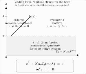
For $d>2$, the regulated large-$N$ model has a critical bare coupling $\alpha_c(\Lambda)=1/[NI_d(0;\Lambda)]$. Below $\alpha_c$ the saddle is ordered and has massless Goldstone modes. Above $\alpha_c$ the saddle is symmetric and massive, with $m=\xi^{-1}$.

As a concrete example, take $d=3$ with a sharp cutoff. Then

$$I_3(m) ={1\over2\pi^2}\left[\Lambda-m\arctan{\Lambda\over m}\right].$$

For $m\ll\Lambda$,

$$I_3(m)=I_3(0)-{m\over4\pi}+O(m^2/\Lambda), \qquad I_3(0)={\Lambda\over2\pi^2}.$$

The critical coupling is

$$\alpha_c={2\pi^2\over N\Lambda}.$$

On the symmetric side, $N\alpha_0 I_3(m)=1$ gives

$$N\alpha_0\left(I_3(0)-{m\over4\pi}+\cdots\right)=1.$$

Using $NI_3(0)\alpha_c=1$, we find

$$m\propto \alpha_0-\alpha_c, \qquad d=3,$$

so

$$m^2\propto(\alpha_0-\alpha_c)^2.$$

This is the large-$N$ critical exponent $\nu=1$ in three dimensions. More generally, for $2<d<4$,

$$I_d(0)-I_d(m)\propto m^{d-2},$$

so

$$m\propto (\alpha_0-\alpha_c)^{1/(d-2)}, \qquad \nu={1\over d-2}$$

at $N=\infty$.

The 2+ε expansion

The lower critical dimension for continuous symmetry breaking is $d=2$. Just above two dimensions, $[\alpha]=2-d=-\epsilon$, so the dimensionful sigma-model coupling can be converted into a weak dimensionless coupling and the model has a perturbative critical point.

Let

$$d=2+\epsilon, \qquad \epsilon>0,$$

and define a dimensionless coupling

$$t(\mu)=\mu^\epsilon\alpha(\mu).$$

To one loop,

$$\boxed{ \beta(t)=\mu{dt\over d\mu} =\epsilon t-c t^2+O(t^3), }$$

where, for the $O(N)$ model in the usual normalization,

$$c={N-2\over2\pi}.$$

The perturbative nonzero fixed point below assumes $N>2$. For $N=2$, $c=0$ because the target circle is locally flat, and the compact vortex sectors require a separate treatment.

The fixed points are

$$t=0, \qquad t_*={\epsilon\over c}+O(\epsilon^2).$$

The nonzero fixed point is the critical point separating the ordered and disordered phases. It is the perturbative version of the large-$N$ critical coupling.

Equivalently, in a cutoff language one finds a running dimensionful coupling of the form

$$\alpha(p)= {\alpha_0\over 1-{c\alpha_0\over\epsilon}(\Lambda^\epsilon-p^\epsilon)}.$$

The critical bare coupling satisfies

$${c\alpha_c\over\epsilon}\Lambda^\epsilon=1.$$

At this value,

$$\alpha(p)={\epsilon\over c}\,{1\over p^\epsilon}, \qquad p^\epsilon\alpha(p)={\epsilon\over c}.$$

Thus the dimensionless coupling sits at the fixed point $t_*$. The formula is the $2+\epsilon$ analog of the logarithmic running in two dimensions: the logarithm

$$\log{\Lambda\over p}$$

is replaced by

$${1\over\epsilon}(\Lambda^\epsilon-p^\epsilon).$$

Two descriptions of the same critical point

The $O(N)$ critical point has two famous perturbative descriptions. Near two dimensions, the natural variables are constrained fields $\mathbf n^2=1$ and the coupling is the sigma-model stiffness. Near four dimensions, the natural variables are unconstrained fields $\boldsymbol\phi$ with a quartic potential,

$$S[\boldsymbol\phi] = \int d^dx\, \left[ {1\over2}(\partial_\mu\boldsymbol\phi)^2 +{r\over2}\boldsymbol\phi^2 +{u\over4!}(\boldsymbol\phi^2)^2 \right].$$

In $d=4-\epsilon$, the quartic coupling has beta function

$$\beta(u)=-\epsilon u+{N+8\over48\pi^2}u^2+O(u^3),$$

so there is a Wilson–Fisher fixed point

$$u_*={48\pi^2\over N+8}\epsilon+O(\epsilon^2).$$

The two expansions are not two different physical systems. They are two coordinate systems on the same $O(N)$ universality class:

$$\text{nonlinear sigma model near }2+\epsilon \quad\longleftrightarrow\quad \phi^4\text{ theory near }4-\epsilon.$$

The sigma-model language makes Goldstone fluctuations and the lower critical dimension transparent. The Landau–Ginzburg language makes the order-parameter amplitude, the mass tuning $r-r_c$, and the upper critical dimension transparent.

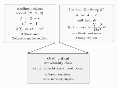
For $N>2$, the $2+\epsilon$ nonlinear sigma model and the $4-\epsilon$ Landau–Ginzburg $\phi^4$ theory are complementary perturbative descriptions of the same $O(N)$ critical universality class.

This is a major lesson of renormalization. A universality class is not identical to a microscopic Lagrangian. Different Lagrangians, even with different-looking fields, can flow to the same long-distance fixed point.

Relation to theta terms

For a one-dimensional antiferromagnetic spin chain, the Euclidean field theory is two-dimensional. The conclusion of this page is therefore immediate:

$$\langle\mathbf n\rangle=0.$$

This does not decide whether the chain is gapped or critical. It only says that the local Néel vector does not condense. The theta term helps decide which symmetry-restored infrared behavior appears. At $\theta=0$, the ordinary $O(3)$ sigma model is massive. At $\theta=\pi$, topological interference together with the spin-chain symmetries can produce the critical $SU(2)_1$ universality class. Thus low-dimensional fluctuations remove conventional order, while topology and global symmetry data distinguish the possible no-order phases.

The next step is to study the topological sectors themselves: maps $S^2\to S^2$, their integer charge, and the instantons that represent them semiclassically.

Summary

Continuous symmetry breaking requires more than a classical manifold of minima. In finite volume, the path integral averages over the global orientation and restores the symmetry. In infinite volume, a pure phase can exist only if long-wavelength Goldstone fluctuations are not too large.

For an attempted $O(N)\to O(N-1)$ breaking pattern, the decisive integral is

$$\int_{1/L}^{\Lambda}{d^dk\over k^2}.$$

It diverges for $d\le2$. Under the equilibrium, locality, and regularity assumptions stated above, this prevents spontaneous breaking of a continuous internal symmetry. This is the infrared heart shared by the Mermin–Wagner–Hohenberg theorem and Coleman’s relativistic result.

At large $N$, the same statement appears in the saddle equation

$$N\alpha_0 I_d(m)=1.$$

For $d\le2$, the model is symmetry-restored for any nonzero coupling. For $d>2$, there is a critical coupling

$$\alpha_c(\Lambda)={1\over NI_d(0;\Lambda)},$$

separating an ordered Goldstone phase from a symmetric massive phase. For $N>2$, the critical point is perturbative in nonlinear-sigma-model variables near $d=2+\epsilon$; near $d=4-\epsilon$, the same universality class is perturbative in $\phi^4$ variables.

Common pitfalls

Confusing a symmetric finite box with the thermodynamic limit. The statement $\langle\mathbf n\rangle=0$ at finite volume assumes symmetric boundary conditions and is not by itself a proof that spontaneous symmetry breaking is impossible. A broken phase is defined by taking $V\to\infty$ before removing the selecting source.

Applying Mermin–Wagner outside its hypotheses. The theorem concerns continuous symmetries under locality and equilibrium assumptions; it does not forbid discrete symmetry breaking. The two-dimensional Ising model is the standard correction to an overbroad slogan.

Equating absence of magnetization with absence of every transition. The two-dimensional $O(2)$ model has no conventional magnetization, but compactness and vortices produce the Berezinskii–Kosterlitz–Thouless transition.

Treating the saddle mass as a microscopic parameter. The mass $m$ is the saddle value $m^2=\lambda$ of the constraint field, not a bare mass inserted into the sigma model. It equals the inverse correlation length in the symmetric phase.

Mixing spatial and Euclidean dimensions. The $d$ in the formulas is total Euclidean dimension. At zero temperature, a one-dimensional quantum antiferromagnet maps to a two-dimensional Euclidean field theory; at nonzero temperature, the original Mermin–Wagner statement counts spatial dimensions.

Exercises

Exercise 1: the infrared divergence of Goldstone modes

Evaluate the infrared behavior of

$$J_d(L)=\int_{1/L}^{\Lambda}{d^dk\over(2\pi)^d}\,{1\over k^2}$$

for $d<2$, $d=2$, and $d>2$.

Solution

Using spherical coordinates in $d$ dimensions,

$$d^dk=S_{d-1}k^{d-1}dk, \qquad S_{d-1}={2\pi^{d/2}\over\Gamma(d/2)}.$$

Therefore

$$J_d(L)={S_{d-1}\over(2\pi)^d}\int_{1/L}^{\Lambda}dk\,k^{d-3}.$$

For $d\ne2$,

$$J_d(L)= {S_{d-1}\over(2\pi)^d} {\Lambda^{d-2}-L^{2-d}\over d-2}.$$

If $d<2$, this grows as

$$J_d(L)\sim {S_{d-1}\over(2\pi)^d}{L^{2-d}\over2-d}.$$

For $d=2$,

$$J_2(L)={1\over2\pi}\int_{1/L}^{\Lambda}{dk\over k} ={1\over2\pi}\log(\Lambda L).$$

For $d>2$, the lower limit gives a finite contribution as $L\to\infty$:

$$J_d(\infty)={S_{d-1}\over(2\pi)^d}{\Lambda^{d-2}\over d-2}.$$

Thus Goldstone fluctuations are infrared divergent for $d\le2$ and infrared finite for $d>2$.

Exercise 2: the critical coupling in the three-dimensional large-N model

For $d=3$, compute

$$I_3(m)=\int_{|k|<\Lambda}{d^3k\over(2\pi)^3}{1\over k^2+m^2},$$

find $\alpha_c$ from $N\alpha_c I_3(0)=1$, and show that $m\propto\alpha_0-\alpha_c$ on the symmetric side.

Solution

In three dimensions,

$$I_3(m)={1\over2\pi^2}\int_0^\Lambda dk\,{k^2\over k^2+m^2}.$$

Since

$${k^2\over k^2+m^2}=1-{m^2\over k^2+m^2},$$

we get

$$I_3(m)={1\over2\pi^2}\left[\Lambda-m\arctan{\Lambda\over m}\right].$$

Thus

$$I_3(0)={\Lambda\over2\pi^2},$$

and

$$\alpha_c={1\over N I_3(0)}={2\pi^2\over N\Lambda}.$$

For $m\ll\Lambda$,

$$\arctan{\Lambda\over m}={\pi\over2}+O(m/\Lambda),$$

so

$$I_3(m)=I_3(0)-{m\over4\pi}+O(m^2/\Lambda).$$

The symmetric saddle equation is

$$N\alpha_0 I_3(m)=1.$$

Using $N\alpha_c I_3(0)=1$,

$$N\alpha_0\left(I_3(0)-{m\over4\pi}+\cdots\right) =N\alpha_c I_3(0).$$

Keeping the leading terms near $\alpha_0=\alpha_c$ gives

$$N I_3(0)(\alpha_0-\alpha_c)-{N\alpha_c\over4\pi}m\approx0.$$

Therefore

$$m\approx {4\pi I_3(0)\over\alpha_c}(\alpha_0-\alpha_c),$$

so $m\propto\alpha_0-\alpha_c$.

Exercise 3: rotor spectrum on the sphere

Consider the one-dimensional sigma model

$$S={1\over2\alpha_0}\int d\tau\,\dot{\mathbf n}^{\,2}, \qquad \mathbf n^2=1.$$

Quantize it as a particle on $S^{N-1}$ and show that the energy levels are

$$E_\ell={\alpha_0\over2}\ell(\ell+N-2), \qquad \ell=0,1,2,\ldots.$$

Why does this imply no spontaneous symmetry breaking?

Solution

The Lagrangian is the kinetic energy of a particle moving on the unit sphere with moment of inertia

$$I={1\over\alpha_0}.$$

The Hamiltonian is the Laplacian on the sphere divided by $2I$:

$$H=-{1\over2I}\Delta_{S^{N-1}} =-{\alpha_0\over2}\Delta_{S^{N-1}}.$$

The spherical harmonics on $S^{N-1}$ obey

$$-\Delta_{S^{N-1}}Y_{\ell}=\ell(\ell+N-2)Y_{\ell}.$$

Hence

$$E_\ell={\alpha_0\over2}\ell(\ell+N-2).$$

The ground state has $\ell=0$ and is the constant wavefunction on $S^{N-1}$. It is an $O(N)$ singlet. Since $\mathbf n$ transforms as a vector, its expectation value in a singlet state vanishes:

$$\langle0|\mathbf n|0\rangle=0.$$

This single quantum rotor has no thermodynamic limit in which a continuum of orientations can become superselected. Its unique singlet ground state therefore does not spontaneously break the continuous $O(N)$ symmetry.

Exercise 4: algebraic order in the two-dimensional O(2) spin-wave theory

For

$$S={1\over2\alpha_0}\int d^2x\,(\partial_\mu\theta)^2,$$

show that

$$\langle e^{i\theta(x)}e^{-i\theta(0)}\rangle \propto |x|^{-\alpha_0/(2\pi)}$$

within the Gaussian spin-wave approximation.

Solution

The Gaussian propagator is

$$\langle\theta(x)\theta(0)\rangle =\alpha_0\int {d^2k\over(2\pi)^2}{e^{ik\cdot x}\over k^2}.$$

With an infrared regulator, the long-distance part is

$$\langle\theta(x)\theta(0)\rangle =-{\alpha_0\over2\pi}\log |x|+\text{constant}.$$

For a Gaussian field,

$$\langle e^{i\theta(x)}e^{-i\theta(0)}\rangle = \exp\left[-{1\over2}\langle(\theta(x)-\theta(0))^2\rangle\right].$$

Now

$$\langle(\theta(x)-\theta(0))^2\rangle =2\left[\langle\theta(0)^2\rangle-\langle\theta(x)\theta(0)\rangle\right] ={\alpha_0\over\pi}\log |x|+\text{constant}.$$

Therefore

$$\langle e^{i\theta(x)}e^{-i\theta(0)}\rangle \propto \exp\left[-{\alpha_0\over2\pi}\log |x|\right] =|x|^{-\alpha_0/(2\pi)}.$$

The correlation decays to zero at large distance, so there is no magnetization, but the decay is algebraic within the spin-wave approximation.

Exercise 5: the 2+ε fixed point

Let the dimensionless sigma-model coupling $t$ obey

$$\beta(t)=\mu{dt\over d\mu}=\epsilon t-c t^2, \qquad c>0.$$

Find the fixed points and the linearized beta function near the nonzero fixed point.

Solution

The fixed points obey

$$0=\epsilon t-c t^2=t(\epsilon-ct).$$

Thus

$$t_0=0, \qquad t_*={\epsilon\over c}.$$

The derivative of the beta function is

$$\beta'(t)=\epsilon-2ct.$$

At the nonzero fixed point,

$$\beta'(t_*)= \epsilon-2c{\epsilon\over c} =-\epsilon.$$

Thus a small perturbation $\delta t=t-t_*$ obeys

$$\mu{d\delta t\over d\mu}=-\epsilon\delta t+O(\delta t^2).$$

This eigenvalue controls the leading departure from criticality in the $2+\epsilon$ expansion.

Because the relevant scaling exponent is $y_t=\epsilon+O(\epsilon^2)$, the corresponding leading correlation-length exponent is

$$\nu={1\over\epsilon}+O(1).$$

References

• Coleman, Sidney. “There Are No Goldstone Bosons in Two Dimensions.” Communications in Mathematical Physics 31 (1973): 259–264. doi:10.1007/BF01646487.
• Hohenberg, Pierre C. “Existence of Long-Range Order in One and Two Dimensions.” Physical Review 158 (1967): 383–386. doi:10.1103/PhysRev.158.383.
• Mermin, N. David, and Herbert Wagner. “Absence of Ferromagnetism or Antiferromagnetism in One- or Two-Dimensional Isotropic Heisenberg Models.” Physical Review Letters 17 (1966): 1133–1136; erratum, 1307. doi:10.1103/PhysRevLett.17.1133.

Further reading

• Altland, Alexander, and Ben Simons. Condensed Matter Field Theory. 3rd ed. Cambridge University Press, 2023.
• Polyakov, Alexander M. Gauge Fields and Strings. Contemporary Concepts in Physics, Vol. 3. Harwood Academic Publishers, 1987.
• Zinn-Justin, Jean. Quantum Field Theory and Critical Phenomena. 5th ed. Oxford University Press, 2021.