QED and Yang–Mills Beta Functions

The previous pages developed three views of vacuum polarization: a momentum-space transverse tensor, a running charge, and a proper-time determinant in a background magnetic field. We now combine them into the one-loop beta functions of Abelian and non-Abelian gauge theory.

The central physical question is deceptively simple: why does QED screen charge while Yang–Mills theory antiscreens it? Charged scalars and fermions polarize the vacuum in a way that weakens long-distance electric fields. Gauge bosons in a non-Abelian theory also carry charge, but their spin-one magnetic moment produces a stronger paramagnetic response with the opposite sign. The final result is asymptotic freedom: at short distances, the Yang–Mills coupling becomes small.

The background-field method computes this coefficient while preserving gauge covariance of the background. One separates a smooth background from the quantum fluctuation and extracts the local ultraviolet correction to its $F^2$ term. This page derives that coefficient in background Feynman gauge, explains the spin decomposition, and states the general one-loop result with matter. The calculation concerns perturbative ultraviolet running; it does not establish a stable chromomagnetic vacuum or an infrared mass gap.

Required background. Effective Actions in Background Fields supplies the proper-time determinants and the orbital-versus-spin decomposition used below. Running Charge, Screening, and Antiscreening fixes the inverse-coupling interpretation of screening. All one-loop results below are translated into $b_0$, defined by $\beta(g)=-b_0g^3/(16\pi^2)+O(g^5)$. One Dirac or Weyl fermion in representation $R$ contributes respectively $-4T(R)/3$ or $-2T(R)/3$; one complex or real scalar contributes $-T(R)/3$ or $-T(R)/6$; and pure Yang–Mills contributes $+11C_A/3$. Thus Abelian matter gives $b_0<0$ and $\beta(e)>0$.

From the F² term to a beta function

Gauge-field and beta-function normalization. The background-field calculation is Euclidean. We use the rescaled gauge-field normalization

$$\boxed{ \Gamma[A]\supset {1\over4}\int d^4x\,{1\over g^2}F^a_{\mu\nu}F^a_{\mu\nu} }$$

or, equivalently, $\Gamma[A]\supset (2g^2)^{-1}\int \operatorname{tr}F_{\mu\nu}F_{\mu\nu}$ when $\operatorname{tr}(T^aT^b)=\delta^{ab}/2$. The coupling sits in front of the gauge kinetic term; covariant derivatives in the fluctuation operator use the rescaled background field.

For Abelian matter of unit charge,

$$D_\mu=\partial_\mu-iA_\mu, \qquad [D_\mu,D_\nu]=-iF_{\mu\nu}.$$

For adjoint non-Abelian fluctuations,

$$\bar D_\mu X=\partial_\mu X+[\bar A_\mu,X], \qquad [\bar D_\mu,\bar D_\nu]X=[\bar F_{\mu\nu},X].$$

Here, only in the adjoint fluctuation formulas, $\bar A_\mu$ denotes the anti-Hermitian connection $\bar A_\mu=-i\bar A^a_{\mu,H}T^a$, and $\bar F_{\mu\nu}=-i\bar F^a_{\mu\nu}T^a$. Thus $\bar D_\mu X=\partial_\mu X-i[\bar A_{\mu,H},X]$ is precisely the Hermitian-generator convention above. The components $\bar F^a_{\mu\nu}$ are real; group invariants below are defined with the Hermitian matrices $T^a$. Relative to an unrescaled Hermitian connection, $\bar A_H=gA_{\mathrm{phys}}$ and $\bar F^a=gF^a_{\mathrm{phys}}$, so the fluctuation curvature carries no additional factor of $g$ in our formulas.

The beta function is

$$\beta(g)=\mu {dg\over d\mu}.$$

We write the Yang–Mills result as

$$\beta(g)=-{b_0\over16\pi^2}g^3+O(g^5).$$

Thus $b_0>0$ means asymptotic freedom.

In the rescaled normalization, the two-point function of the background gauge field defines the running inverse coupling. For an Abelian field in Euclidean momentum space,

$$\Gamma^{(2)}[A] ={1\over2}\int_q A_\mu(-q) \left(q^2\delta_{\mu\nu}-q_\mu q_\nu\right) {1\over e^2(q)}A_\nu(q)+\cdots.$$

The transverse tensor is forced by gauge invariance. The entire one-loop question is the coefficient of the logarithm in $1/e^2(q)$.

For $N_f$ Dirac fermions and $N_s$ charged complex scalars of unit Abelian charge,

$${1\over e^2(q)} ={1\over e^2(\mu)} +{1\over16\pi^2} \left({4\over3}N_f+{1\over3}N_s\right) \log{\mu^2\over q^2}.$$

Only the one-loop logarithm is displayed; finite matching terms depend on the definition of the effective charge, and higher-loop corrections begin at the next order in $e^2$. Differentiating at fixed bare coupling gives

$$\boxed{ \beta_{\mathrm{QED}}(e) ={e^3\over16\pi^2} \left({4\over3}N_f+{1\over3}N_s\right)+O(e^5). }$$

The sign is positive. As the renormalization scale $\mu$ is raised, the charge increases. Equivalently, at longer distances the charge is screened.

For Yang–Mills theory it is more natural to write

$${1\over g^2(q)} ={1\over g^2(\mu)} +{b_0\over16\pi^2}\log{q^2\over\mu^2},$$

so that

$$\boxed{ \beta(g)=-{b_0\over16\pi^2}g^3+O(g^5). }$$

The sign has reversed relative to QED if $b_0>0$: the inverse coupling grows in the ultraviolet, so the coupling itself shrinks.

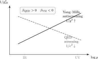
QED screening and Yang–Mills antiscreening in the inverse-coupling language. At one loop, $1/e^2$ decreases toward the ultraviolet, while $1/g^2$ in pure Yang–Mills increases toward the ultraviolet.

The coefficient being computed is that of the transverse background-field kinetic term. Background gauge covariance constrains its form; the full off-shell effective action can still depend on the gauge parameter used for the quantum fluctuation. It is not itself a physical observable. The distinction and the relation to coupling renormalization are developed in Background-Field Yang–Mills Effective Action.

Here is the sign dictionary used in the rest of the course:

$$\begin{array}{c|c|c} \text{theory} & \text{UV behavior of }1/g^2(\mu) & \text{UV behavior of }g(\mu) \\ \hline \text{QED matter} & \text{decreases} & \text{increases} \\ \text{pure Yang–Mills} & \text{increases} & \text{decreases} \end{array}$$

Most sign mistakes in this calculation come from silently switching between $g$, $g^2$, and $1/g^2$.

This statement is also why the background-field method is more than a shortcut. In ordinary gauges one separately computes wavefunction, vertex, and coupling counterterms. In background-field gauge, background gauge invariance ties the renormalization of the background two-point function directly to the coupling renormalization.

Matter loops: scalar and spinor screening

The matter coefficients can be read directly from the proper-time result of the previous page. A complex scalar in a constant magnetic field gives

$$\Delta\left({1\over e^2}\right)_s ={1\over16\pi^2}{1\over3}\log {\Lambda^2\over m^2}.$$

A Dirac fermion gives

$$\Delta\left({1\over e^2}\right)_f ={1\over16\pi^2}{4\over3}\log {\Lambda^2\over m^2}.$$

The scalar contribution is orbital. The fermion contribution contains both orbital motion and the Pauli spin coupling. In the magnetic-field heat kernel, this distinction appears in the expansion

$$4{x\over\sinh x}\cosh x =4\left(1-{x^2\over6}+\cdots\right) \left(1+{x^2\over2}+\cdots\right) =4+{4\over3}x^2+\cdots.$$

The $-2/3$ orbital piece and the $+2$ spin piece add to $4/3$:

$$-{2\over3}+2={4\over3}.$$

Both scalar and fermion matter screen. In a non-Abelian theory, matter fields still screen. The only new ingredient is the group-theory weight.

Let $R$ be a representation of the gauge group, with Hermitian generators normalized by

$$\operatorname{tr}_R(T^aT^b)=T_R\delta^{ab}.$$

Then one Dirac fermion in $R$ contributes

$$\Delta b_0^{\mathrm{Dirac}}=-{4\over3}T_R,$$

and one complex scalar in $R$ contributes

$$\Delta b_0^{\mathrm{complex\ scalar}}=-{1\over3}T_R.$$

The minus signs appear because $b_0$ is defined by $\beta(g)=-b_0g^3/(16\pi^2)$. Matter has the QED sign, so it reduces $b_0$ and pushes the theory away from asymptotic freedom. This is often the cleanest way to remember the formula: gauge bosons add to $b_0$, ordinary matter subtracts from $b_0$.

For a real scalar the coefficient is half as large,

$$\Delta b_0^{\mathrm{real\ scalar}}=-{1\over6}T_R,$$

and for a Weyl fermion it is half a Dirac fermion,

$$\Delta b_0^{\mathrm{Weyl}}=-{2\over3}T_R.$$

These factors are often the easiest way to check supersymmetric cancellations.

Background-field expansion of Yang–Mills theory

Now consider pure Yang–Mills theory. Write the gauge field as a background plus a quantum fluctuation,

$$A_\mu=\bar A_\mu+a_\mu.$$

The field strength expands as

$$F_{\mu\nu}[\bar A+a] =\bar F_{\mu\nu} +\bar D_\mu a_\nu-\bar D_\nu a_\mu +[a_\mu,a_\nu].$$

A background gauge transformation acts by

$$\bar A_\mu\mapsto h^{-1}\bar A_\mu h+h^{-1}\partial_\mu h, \qquad a_\mu\mapsto h^{-1}a_\mu h.$$

Thus the background is a connection, while the fluctuation transforms homogeneously. The gauge condition

$$\bar D_\mu a_\mu=0$$

preserves background gauge invariance. This is the reason the method is so efficient: the effective action generated for $\bar A_\mu$ must be a gauge-invariant functional of the background.

Expanding the Yang–Mills action to quadratic order in $a_\mu$ and adding background Feynman gauge fixing gives the vector fluctuation operator

$$\mathcal L_{\mu\nu}^{\mathrm{vec}} =-\bar D^2\delta_{\mu\nu}-2\operatorname{ad}(\bar F_{\mu\nu}),$$

where

$$\operatorname{ad}(\bar F_{\mu\nu})X=[\bar F_{\mu\nu},X].$$

The Faddeev–Popov ghosts are Grassmann scalar fields in the adjoint representation with operator

$$\mathcal L_{\mathrm{gh}}=-\bar D^2.$$

Therefore the one-loop effective action is schematically

$$\boxed{ \Gamma^{(1)}_{\mathrm{YM}}[\bar A] ={1\over2}\operatorname{Tr}_{1,\mathrm{adj}}\log \left(-\bar D^2\delta_{\mu\nu}-2\operatorname{ad}\bar F_{\mu\nu}\right) -\operatorname{Tr}_{0,\mathrm{adj}}\log(-\bar D^2). }$$

The factor $1/2$ is the Gaussian determinant of a real bosonic vector field. The ghost and antighost form one independent Grassmann pair per adjoint component, giving a determinant with weight $-1$, not $-1/2$. The vector trace includes Lorentz-vector indices and adjoint color indices; the ghost trace includes only adjoint color indices. These are the unrestricted vector and ghost determinants in background Feynman gauge, as in Vassilevich 2003, §3.4, pp.27–28, Eqs.(3.46), (3.49), (3.51)–(3.53), preprint PDF. A strictly transverse vector determinant has a different ghost power and must not be substituted into this formula.

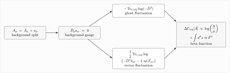
The background-field split $A=\bar A+a$ preserves manifest gauge covariance in the background. Gauge fluctuations contribute a spin-one determinant, while ghosts contribute scalar adjoint determinants that remove unphysical gauge modes.

The CP-even logarithmic divergence quadratic in a slowly varying background must be proportional to

$$\int d^4x\,\bar F^a_{\mu\nu}\bar F^a_{\mu\nu},$$

up to total derivatives. The other familiar dimension-four gauge invariant, $\operatorname{tr}\bar F_{\mu\nu}\widetilde{\bar F}_{\mu\nu}$, is CP odd and topological, so it is not generated by this CP-even fluctuation determinant. Extracting the coefficient of $\bar F^2$ gives the beta function.

Computing the ultraviolet heat coefficient

Take a smooth background in flat Euclidean space and a compact simple gauge group. Use a periodic box, or sufficient falloff to discard integrated total derivatives. We need only the short-proper-time expansion. A finite upper cutoff $s_{\mathrm{IR}}$ separates it from possible zero or negative modes of the vector operator; no convergence of the full integral at $s\to\infty$ is assumed. The distinction between ultraviolet coefficients and infrared convergence is explicit in Vassilevich 2003, §1, pp.7–8, Eqs.(1.16)–(1.21), preprint PDF.

Write an operator of Laplace type as

$$P=-(\bar D^2+E), \qquad \Omega_{\mu\nu}=[\bar D_\mu,\bar D_\nu].$$

For its diagonal heat trace in four flat dimensions,

$$\begin{aligned} \operatorname{Tr}e^{-sP} \sim {1\over(4\pi s)^2}\int d^4x\, \operatorname{tr}\Bigl[\mathbf 1+sE +s^2\Bigl({E^2\over2} +{\Omega_{\mu\nu}\Omega_{\mu\nu}\over12} +{\bar D^2E\over6}\Bigr)+\cdots\Bigr]. \end{aligned}$$

Here $\operatorname{Tr}$ includes the spacetime integration, whereas $\operatorname{tr}$ acts on the finite internal indices. This local expansion, with exactly the sign convention for $P$ above, is Vassilevich 2003, §2.1, p.11, Eq.(2.2), and §4.1, pp.39–40, Eqs.(4.25), (4.28), preprint PDF. It is the mathematical input we use; a general proof for curved spaces or boundaries is outside this lesson. Heat Kernels, Zeta Functions, and Spectral Determinants explains the broader operator assumptions.

The two coefficients relevant here also have simple checks. A constant commuting $E$ multiplies the free heat kernel by $e^{sE}$, fixing the $E^2/2$ term. For a unit-charge scalar with $F_{12}=B$, the previous lesson gave

$${Bs\over\sinh Bs}=1-{B^2s^2\over6}+O(s^4).$$

Since $\Omega_{12}=-iB$ and both ordered index pairs occur, $\Omega_{\mu\nu}\Omega_{\mu\nu}=-2B^2$. Thus the curvature coefficient is $1/12$. Gauge covariance and dimensional counting leave precisely these two quadratic invariants, plus a total derivative, in this flat CP-even coefficient.

Define

$$\mathcal Q=C_A\bar F^a_{\mu\nu}\bar F^a_{\mu\nu}, \qquad \operatorname{tr}_{\mathrm{adj}}(T^a_{\mathrm{adj}}T^b_{\mathrm{adj}}) =C_A\delta^{ab}.$$

Because $\Omega_{\mu\nu}=-i\bar F^a_{\mu\nu}T^a_{\mathrm{adj}}$, its color trace has a minus sign:

$$\operatorname{tr}_{\mathrm{adj}} \Omega_{\mu\nu}\Omega_{\mu\nu}=-\mathcal Q.$$

For the vector operator, $E_{\mu\nu}=2\Omega_{\mu\nu}$. The connection acts identically on each of the four vector components, but $E$ mixes them. Therefore

$$\begin{aligned} \operatorname{tr}_{1,\mathrm{adj}}\Omega^2&=-4\mathcal Q,\\ \operatorname{tr}_{1,\mathrm{adj}}E^2 &=4\sum_{\mu,\nu}\operatorname{tr}_{\mathrm{adj}} \Omega_{\mu\nu}\Omega_{\nu\mu} =4\mathcal Q. \end{aligned}$$

The second sign uses $\Omega_{\nu\mu}=-\Omega_{\mu\nu}$; treating $E^2$ as four unrelated scalar squares would miss it. For the ghost, $E=0$ and only the color trace remains. After the total derivative is integrated out, denote the coefficient without $(4\pi)^{-2}$ by $h_4$:

$$\begin{aligned} h_4^{\mathrm{vec}} &=-{4\mathcal Q\over12}+{4\mathcal Q\over2} ={5\over3}\mathcal Q,\\ h_4^{\mathrm{gh}}&=-{\mathcal Q\over12},\\ H_4\equiv {1\over2}h_4^{\mathrm{vec}}-h_4^{\mathrm{gh}} &={11\over12}\mathcal Q. \end{aligned}$$

This is the decisive vector-and-ghost trace calculation. Vassilevich 2003, §4.2.1, pp.40–41, Eqs.(4.30)–(4.34), preprint PDF obtains the same result, but defines his integrated total heat coefficient as $a_4^{\mathrm{vec}}-2a_4^{\mathrm{gh}}$. That convention is twice $(16\pi^2)^{-1}\int d^4x\,H_4$, because our coefficient includes the real-vector Gaussian weight.

From the pole to the coupling flow

The proper-time identity contributes a further minus sign:

$$\Gamma^{(1)}_{\mathrm{UV}} =-\int_0^{s_{\mathrm{IR}}}{ds\over s} \left({1\over2}\operatorname{Tr}e^{-s\mathcal L_{\mathrm{vec}}} -\operatorname{Tr}e^{-s\mathcal L_{\mathrm{gh}}}\right).$$

This expression denotes its ultraviolet part, with a regulator at the lower endpoint and background-independent terms subtracted. In $d=4-2\epsilon$, the $F^2$ term contains $\int_0^{s_{\mathrm{IR}}}ds\,s^{-1+\epsilon}$, whose pole is $1/\epsilon$. Four vector components suffice for this pole; their $O(\epsilon)$ correction contributes only to finite terms. Hence

$$\Gamma^{(1)}_{\mathrm{div}} =-{\mu^{-2\epsilon}\over16\pi^2\epsilon} {11C_A\over12} \int d^dx\,\bar F^a_{\mu\nu}\bar F^a_{\mu\nu}.$$

Canceling it with the bare kinetic term requires

$${1\over g_0^2} =\mu^{-2\epsilon} \left[{1\over g^2}+{b_0\over16\pi^2\epsilon}+\cdots\right], \qquad b_0={11\over3}C_A.$$

The factor four comes from the normalization $F^2/(4g_0^2)$. Differentiate at fixed $g_0$, retaining the dimensional part of $\beta_d=\mu\,dg/d\mu$:

$$\begin{aligned} 0&=-{2\epsilon\over g^2}-{2b_0\over16\pi^2} -{2\beta_d\over g^3}+O(g^2),\\ \beta_d&=-\epsilon g-{b_0g^3\over16\pi^2}+O(g^5). \end{aligned}$$

Taking $\epsilon\to0$ yields the advertised negative Yang–Mills beta function. As a diagrammatic check, the separate background-gauge ghost and vector contributions give $C_A/3$ and $10C_A/3$ to $b_0$ in Schwartz 2014, §34.3.2, pp.756–757, Eqs.(34.96), (34.101). His dimensional parameter is $\epsilon_{\mathrm S}=2\epsilon$ because he uses $d=4-\epsilon_{\mathrm S}$; the pole and fixed-bare calculation above specify our normalization directly.

Spin-one paramagnetism and the coefficient eleven-thirds

The operator

$$-\bar D^2\delta_{\mu\nu}$$

is the orbital part. If this were the whole story, a gauge boson would resemble several charged scalar fields in the adjoint representation and would screen the charge. The crucial term is

$$-2\operatorname{ad}(\bar F_{\mu\nu}).$$

This is the spin-one magnetic-moment coupling. It is the vector analog of the Pauli term in the squared Dirac operator. Its effect has the opposite sign and is larger.

A clean comparison uses one quantity throughout. Write the one-loop contribution of a field species as

$$\beta(g)=c\,{g^3\over16\pi^2}+O(g^5).$$

For one complex scalar, $c/T_R=+1/3$. For one Dirac fermion, the orbital and Pauli contributions to $c/T_R$ give

$$-{2\over3}+2={4\over3}.$$

For the pure Yang–Mills gauge-and-ghost sector, the orbital terms in $H_4$ are $\tfrac12(-\mathcal Q/3)-(-\mathcal Q/12)=-\mathcal Q/12$, while the vector spin term is $\tfrac12(2\mathcal Q)=\mathcal Q$. Since $c=-b_0$ and $b_0$ is four times the coefficient of $\bar F^a\bar F^a$ in $H_4$, this gives

$${c\over C_A}=\underbrace{{1\over3}}_{\text{orbital}} +\underbrace{(-4)}_{\text{spin-one moment}} =-{11\over3}.$$

Multiplying by $2g$ converts this to the coefficient in the flow of $g^2$:

$${d g^2\over d\log\mu}=2g\beta(g),$$

so the same pure-gauge decomposition becomes

$${2\over3}-8=-{22\over3}.$$

Thus

$$\boxed{ \beta_{\mathrm{pure\ YM}}(g) =-{g^3\over16\pi^2}{11\over3}C_A+O(g^5). }$$

Ghosts are essential in the actual calculation. They do not merely “subtract two polarizations” in a naive way; rather, they enforce gauge invariance and cancel the unphysical pieces of the vector determinant. A quick check on any derivation is that the final logarithmic divergence must be proportional to the background-gauge-invariant operator $\int \bar F^2$, with no leftover gauge-parameter dependence. But after the dust settles, the physical mnemonic is reliable:

$$\text{spin-one paramagnetism dominates orbital screening.}$$

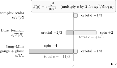
Schematic orbital and spin contributions to $\beta(g)=c\,g^3/(16\pi^2)$ in the background Feynman-gauge calculation. Each row shows the coefficient after its group factor has been removed: $c/T_R$ for matter and $c/C_A$ for Yang–Mills. The labeled numbers, including the row totals, use that normalization; bar lengths are approximate. Scalar and spinor matter screen, while the gauge-and-ghost sum gives $c=-11C_A/3$.

The group factor is

$$f^{acd}f^{bcd}=C_A\delta^{ab},$$

so for $SU(N)$,

$$C_A=N.$$

This is why the pure $SU(N)$ beta function is

$$\beta(g)=-{11N\over3}{g^3\over16\pi^2}+O(g^5).$$

General one-loop result with matter

Combining gauge, fermion, and scalar loops gives

$$\boxed{ \beta(g)=-{g^3\over16\pi^2} \left[ {11\over3}C_A -{4\over3}\sum_{\mathrm{Dirac\ f}}T(R_f) -{1\over3}\sum_{\mathrm{complex\ s}}T(R_s) \right]+O(g^5). }$$

Equivalently, for Weyl fermions and real scalars,

$$\boxed{ b_0={11\over3}C_A -{2\over3}\sum_{\mathrm{Weyl\ f}}T(R_f) -{1\over6}\sum_{\mathrm{real\ s}}T(R_s). }$$

For a chiral matter list, this coefficient presupposes a consistent anomaly-free gauge theory; the numerical beta coefficient alone does not check gauge-anomaly cancellation.

For $SU(N)$ with $N_f$ Dirac fermions in the fundamental representation,

$$T_F={1\over2}, \qquad C_A=N,$$

so

$$\boxed{ b_0={11\over3}N-{2\over3}N_f. }$$

The condition for one-loop asymptotic freedom is

$$b_0>0.$$

For QCD with gauge group $SU(3)$, this condition is

$$11-{2\over3}N_f>0, \qquad N_f<{33\over2}.$$

Thus a small enough number of quark flavors preserves asymptotic freedom. Matter screens, but the gauge field antiscreens more strongly.

Because $N_f$ is an integer, an $SU(3)$ theory with fundamental Dirac fermions is asymptotically free at one loop for $N_f\leq16$.

These formulas assume that the matter fields are light compared with the renormalization scale. If a field has mass $M$, it contributes to the running above $M$ and decouples from low-energy logarithms below $M$ after matching. In a mass-independent subtraction scheme this decoupling is not automatic in the beta function; it is implemented by an effective field theory with threshold matching.

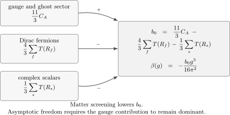
The one-loop coefficient $b_0$ receives a positive contribution from gauge bosons and negative contributions from matter. In the convention $\beta(g)=-b_0g^3/(16\pi^2)$, positive $b_0$ means asymptotic freedom.

The important conceptual point is that the sign of a beta function is not determined merely by whether particles are bosons or fermions. It is determined by the full fluctuation operator: statistics, number of degrees of freedom, representation under the gauge group, and spin coupling to the background field all matter.

For reference, in the convention above:

$$\begin{array}{c|c} \text{field in representation }R & \text{contribution to }b_0 \\ \hline \text{Dirac fermion} & -{4\over3}T(R) \\ \text{Weyl fermion} & -{2\over3}T(R) \\ \text{complex scalar} & -{1\over3}T(R) \\ \text{real scalar} & -{1\over6}T(R) \end{array}$$

This small table is a useful guardrail when moving between particle-physics, supersymmetry, and statistical-field-theory normalizations.

Supersymmetric cancellations and the special role of ten dimensions

The coefficients above give quick checks of supersymmetric gauge theories. In four-dimensional $\mathcal N=4$ super-Yang–Mills theory all fields are in the adjoint representation. The field content can be written as

$$\text{one gauge boson} \quad+ 4\ \text{Weyl fermions} \quad+ 6\ \text{real scalars}.$$

Using $T(\mathrm{adj})=C_A$, the one-loop coefficient is

$$b_0 ={11\over3}C_A -{2\over3}(4C_A) -{1\over6}(6C_A).$$

Therefore

$$\boxed{ b_0=\left({11\over3}-{8\over3}-1\right)C_A=0. }$$

This cancellation is not an accident of arithmetic. Four-dimensional $\mathcal N=4$ super-Yang–Mills can be obtained by dimensional reduction of ten-dimensional minimal supersymmetric Yang–Mills theory. Here we have checked its one-loop gauge beta function; an all-orders conclusion requires additional supersymmetric arguments.

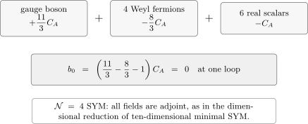
In $\mathcal N=4$ super-Yang–Mills theory, the gauge-boson contribution to $b_0$ is exactly canceled by four adjoint Weyl fermions and six adjoint real scalars: $11/3-8/3-1=0$.

A related mnemonic is that the one-loop coefficient for dimensionally reduced supersymmetric Yang–Mills theories knows about the critical dimension $D=10$. The four-dimensional $\mathcal N=4$ theory inherits precisely the field content of ten-dimensional minimal SYM, and the one-loop gauge beta function vanishes. This remark should not be confused with a proof of all-order finiteness; it is only the one-loop statement visible from the beta-function coefficients on this page.

Solving the asymptotically free flow

For a theory with

$$\beta(g)=-{b_0\over16\pi^2}g^3, \qquad b_0>0,$$

we have

$${d\over d\log\mu}{1\over g^2} =-{2\over g^3}\beta(g) ={b_0\over8\pi^2}.$$

Integrating between $\mu_0$ and $\mu$ gives

$$\boxed{ {1\over g^2(\mu)} ={1\over g^2(\mu_0)}+{b_0\over8\pi^2}\log{\mu\over\mu_0}. }$$

Thus $g(\mu)$ becomes small when $\mu$ becomes large. Perturbation theory improves in the ultraviolet.

The same equation can be written in terms of the RG-invariant scale

$$\Lambda =\mu\exp\left[-{8\pi^2\over b_0g^2(\mu)}\right].$$

Then

$$\boxed{ g^2(\mu) ={8\pi^2\over b_0\log(\mu/\Lambda)} }$$

at one loop. This formula is trustworthy only when $\mu\gg\Lambda$. As $\mu$ approaches $\Lambda$, perturbation theory breaks down. The next page develops this phenomenon as dimensional transmutation: the classical theory has a dimensionless coupling, but the quantum theory produces a scale.

Summary

The beta function of a gauge theory is encoded in the logarithmic renormalization of the background $F^2$ term. In the rescaled normalization, matter loops correct $1/g^2$ directly.

For QED matter,

$$\beta(e)={e^3\over16\pi^2} \left({4\over3}N_f+{1\over3}N_s\right)+O(e^5),$$

so the Abelian charge is screened in the infrared and grows toward the ultraviolet.

For pure Yang–Mills theory,

$$\beta(g)=-{g^3\over16\pi^2}{11\over3}C_A+O(g^5),$$

so the coupling decreases at short distances. The physical origin of the sign is spin-one paramagnetism: the gauge boson magnetic-moment term dominates the orbital screening part. Ghosts are required for the gauge-invariant coefficient.

With matter,

$$b_0={11\over3}C_A -{4\over3}\sum_{\mathrm{Dirac\ f}}T(R_f) -{1\over3}\sum_{\mathrm{complex\ s}}T(R_s).$$

Matter reduces $b_0$. A non-Abelian theory is asymptotically free when the gauge-boson term wins.

Common pitfalls

Inferring the sign from statistics alone. The sign comes from the full quadratic operator in the background field. Spin couplings are decisive.

Dropping the ghost determinant. The background-field vector determinant by itself contains unphysical gauge modes. The ghost determinant is part of the gauge-fixed definition of the theory and is necessary for the coefficient $11/3$.

Mixing the flows of $g$ and $g^2$. If

$$\beta(g)=-{11\over3}{C_Ag^3\over16\pi^2},$$

then

$${d g^2\over d\log\mu}=-{22\over3}{C_Ag^4\over16\pi^2}.$$

The extra factor of two is a common source of mismatched coefficients.

Taking “antiscreening” too literally. A color-charge cloud is not by itself a gauge-invariant observable. The coefficient derived here governs perturbative short-distance running and can enter predictions for specified physical observables. Background gauge covariance alone does not identify the full off-shell effective action with such an observable, or establish the stability of a constant chromomagnetic field.

Exercises

Exercise 1: Derive the QED beta function from the inverse coupling

Starting from

$${1\over e^2(q)}={1\over e^2(\mu)}+{b\over16\pi^2}\log{\mu^2\over q^2},$$

derive

$$\beta(e)={b\over16\pi^2}e^3.$$

Solution

Hold the physical momentum $q$ fixed and differentiate the stated relation with respect to $\log\mu$. The effective coupling on the left is independent of the arbitrary subtraction point, so

$$0=-{2\over e^3}\beta(e)+{2b\over16\pi^2}.$$

Solving gives

$$\boxed{ \beta(e)={b\over16\pi^2}e^3. }$$

Exercise 2: Translate the Yang–Mills flow from the coupling to its square

For pure Yang–Mills theory,

$$\beta(g)=-{11\over3}{C_Ag^3\over16\pi^2}.$$

Find $d g^2/d\log\mu$ and explain why the coefficient is $-22C_A/3$ rather than $-11C_A/3$.

Solution

Use

$${d g^2\over d\log\mu}=2g{dg\over d\log\mu}=2g\beta(g).$$

Substituting the beta function,

$${d g^2\over d\log\mu} =2g\left[-{11\over3}{C_Ag^3\over16\pi^2}\right] =-{22\over3}{C_Ag^4\over16\pi^2}.$$

The coefficient doubles because $g^2$ changes twice as fast logarithmically as $g$:

$${d\log g^2\over d\log\mu}=2{d\log g\over d\log\mu}.$$

Exercise 3: Find the asymptotic-freedom window for fundamental matter

For $SU(N)$ gauge theory with $N_f$ Dirac fermions in the fundamental representation and no scalars, show that

$$b_0={11\over3}N-{2\over3}N_f.$$

For what values of $N_f$ is the theory asymptotically free?

Solution

For $SU(N)$,

$$C_A=N, \qquad T_F={1\over2}$$

in the fundamental representation. The general formula with $N_f$ Dirac fermions is

$$b_0={11\over3}C_A-{4\over3}T_FN_f.$$

Substituting the group factors gives

$$b_0={11\over3}N-{4\over3}{1\over2}N_f ={11\over3}N-{2\over3}N_f.$$

Asymptotic freedom requires $b_0>0$, so

$${11\over3}N-{2\over3}N_f>0.$$

Multiplying by $3$ gives

$$11N-2N_f>0,$$

hence

$$\boxed{N_f<{11\over2}N.}$$

For $SU(3)$ this becomes $N_f<33/2$.

Exercise 4: Check the maximally supersymmetric one-loop cancellation

Check the one-loop cancellation in $\mathcal N=4$ super-Yang–Mills theory. Use one gauge boson, four Weyl fermions, and six real scalars, all in the adjoint representation.

Solution

For adjoint fields,

$$T(\mathrm{adj})=C_A.$$

The gauge boson contributes

$${11\over3}C_A.$$

Each Weyl fermion contributes

$$-{2\over3}C_A,$$

so four Weyl fermions contribute

$$4\left(-{2\over3}C_A\right)=-{8\over3}C_A.$$

Each real scalar contributes

$$-{1\over6}C_A,$$

so six real scalars contribute

$$6\left(-{1\over6}C_A\right)=-C_A.$$

The total coefficient is

$$b_0={11\over3}C_A-{8\over3}C_A-C_A =\left({11\over3}-{8\over3}-{3\over3}\right)C_A=0.$$

Thus the one-loop beta function vanishes.

Exercise 5: Construct the one-loop RG-invariant scale

Let

$$\beta(g)=-{b_0\over16\pi^2}g^3, \qquad b_0>0.$$

Show that

$$\Lambda=\mu\exp\left[-{8\pi^2\over b_0g^2(\mu)}\right]$$

is independent of $\mu$ at one loop.

Solution

First compute the flow of the inverse coupling:

$${d\over d\log\mu}{1\over g^2} =-{2\over g^3}\beta(g) ={b_0\over8\pi^2}.$$

Now take the logarithm of $\Lambda$:

$$\log\Lambda=\log\mu-{8\pi^2\over b_0g^2(\mu)}.$$

Differentiate:

$${d\log\Lambda\over d\log\mu} =1-{8\pi^2\over b_0}{d\over d\log\mu}{1\over g^2(\mu)}.$$

Using the inverse-coupling flow,

$${d\log\Lambda\over d\log\mu} =1-{8\pi^2\over b_0}{b_0\over8\pi^2}=0.$$

Therefore $\Lambda$ is RG invariant at one loop.

Exercise 6: Test the ghost weight in the heat coefficient

Use $h_4^{\mathrm{vec}}=5\mathcal Q/3$ and $h_4^{\mathrm{gh}}=-\mathcal Q/12$ to find the inferred $b_0$ if the ghost determinant is (a) omitted or (b) mistakenly assigned weight $-1/2$. Explain why neither reproduces Yang–Mills theory.

Solution

Write $H_4=\mathcal Q h$. The kinetic normalization gives $b_0=4C_Ah$. Without the ghost,

$$h={1\over2}{5\over3}={5\over6}, \qquad b_0={10\over3}C_A.$$

With half the required ghost weight,

$$h={5\over6}+{1\over24}={7\over8}, \qquad b_0={7\over2}C_A.$$

The actual Grassmann pair has weight $-1$, giving $h=5/6+1/12=11/12$ and $b_0=11C_A/3$. The ghost operator acts on adjoint scalar components, but its determinant weight follows from Grassmann integration; it cannot be chosen by counting transverse polarizations in the unrestricted vector operator.

References

• Schwartz, Matthew D. Quantum Field Theory and the Standard Model. Cambridge University Press, 2014. DOI. The diagrammatic comparison uses §34.3.2, Eqs.(34.96) and (34.101), with the dimensional-parameter translation stated above.
• Vassilevich, Dmitri V. “Heat Kernel Expansion: User’s Manual.” Physics Reports 388 (2003): 279–360. DOI. Open PDF, arXiv:hep-th/0306138v3. All page locators above refer to this preprint’s printed pagination.

Further reading

• Abbott, L. F. “Introduction to the Background Field Method.” Acta Physica Polonica B 13, no. 1 (1982): 33–50.
• Gross, David J., and Frank Wilczek. “Ultraviolet Behavior of Non-Abelian Gauge Theories.” Physical Review Letters 30, no. 26 (1973): 1343–1346.
• Politzer, H. David. “Reliable Perturbative Results for Strong Interactions?” Physical Review Letters 30, no. 26 (1973): 1346–1349.
• Polyakov, Alexander M. Gauge Fields and Strings. Chur: Harwood Academic Publishers, 1987, Chapter 2.
• Srednicki, Mark. Quantum Field Theory. Cambridge: Cambridge University Press, 2007, Sections 66, 73, and 78.
• Weinberg, Steven. The Quantum Theory of Fields. Volume II: Modern Applications. Cambridge: Cambridge University Press, 1996, Chapters 17–18.
• Zinn-Justin, Jean. Quantum Field Theory and Critical Phenomena. 4th ed. Oxford: Clarendon Press, 2002.