Fermi-Surface Instabilities and One-Dimensional Fermions

The previous page built the field theory of a finite-density Fermi gas. The key lesson was geometric: low-energy modes do not sit near $\mathbf p=0$, but near the Fermi surface $\xi_{\mathbf p}=0$. In dimensions $d>1$, the Fermi surface has many patches, and most small perturbations only connect a small part of the surface to another small part. In one spatial dimension the geometry collapses to two points,

$$p=+p_F, \qquad p=-p_F.$$

That collapse makes the theory much more singular. A momentum transfer near $2p_F$ maps one Fermi point to the other. A particle-hole pair can be made with arbitrarily small energy at a fixed nonzero momentum. This is the kinematic heart of the Peierls instability, charge-density-wave tendencies, spin-density-wave tendencies, and the broader statement that the naive Fermi-gas fixed point in one dimension is precarious.

The point of this page is not yet to solve one-dimensional fermions completely. That will eventually require bosonization and the special structure of two-dimensional field theory. Here we do something more basic and more diagnostic: we compute the free response functions and identify the logarithms that tell us which perturbations cannot be ignored.

Required background. Fermi surface and nonrelativistic many-body fields supplies the filled-sea propagator, the particle-hole bubble, and the response-sign convention used throughout this page. The one-dimensional singularity comes from perfect nesting, not merely from having fewer momentum states: the two Fermi points have opposite velocities, and a single transfer $2p_F$ connects all low-energy right-left particle-hole pairs. That kinematic degeneracy converts a phase-space restriction into a logarithm.

Nested Fermi points

Linearized one-dimensional conventions. We work mostly with spinless fermions to keep factors transparent. A spin degeneracy $g_s$ multiplies free density response functions by $g_s$, but spinful interactions have additional charge and spin channels.

The microscopic dispersion is

$$\xi_p={p^2\over2m}-\mu, \qquad p_F=\sqrt{2m\mu}, \qquad v_F={p_F\over m}.$$

Near the two Fermi points,

$$\psi(x)=e^{ip_Fx}\psi_R(x)+e^{-ip_Fx}\psi_L(x),$$

with slowly varying right- and left-moving fields. The leading real-time action is

$$S_0=\int dt\,dx\, \left[ \psi_R^\dagger(i\partial_t+i v_F\partial_x)\psi_R + \psi_L^\dagger(i\partial_t-i v_F\partial_x)\psi_L \right].$$

A potential energy $U$ couples as $H_{\rm ext}=\int dx\,U\rho$. With this sign convention, the static response of a free gas is negative: a positive potential energy lowers the density.

In one dimension the filled Fermi sea is the interval $-p_F<p<p_F$. Low-energy particles lie just outside the endpoints, while low-energy holes lie just inside them. There are two especially important ways to make soft particle-hole pairs.

First, a small momentum transfer $q\approx0$ moves a fermion within the same Fermi point. This is the smooth-density channel. Second, a momentum transfer

$$q\approx 2p_F$$

moves a fermion from the left Fermi point to the right Fermi point, or conversely from right to left for $q\approx -2p_F$. This is the nested particle-hole channel.

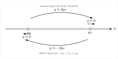
In one dimension the Fermi surface consists of two points. A small momentum transfer moves a state from just inside to just outside one endpoint; a transfer near $2p_F$ does the same while mapping the left endpoint to the right one.

The word nesting means that a single momentum transfer maps an extended set of gapless states into another set of gapless states. In one dimension the “extended set” is just the two endpoints, but the nesting is perfect: the left endpoint and the right endpoint have opposite velocities and are separated by $2p_F$. This perfect kinematic match is what turns ordinary response into logarithmic response.

The density operator makes the same decomposition. Substitute

$$\psi=e^{ip_Fx}\psi_R+e^{-ip_Fx}\psi_L$$

into $\rho=\psi^\dagger\psi$. One obtains

$$\boxed{ \rho(x)=\rho_R(x)+\rho_L(x) +e^{-2ip_Fx}\mathcal O_{2p_F}(x) +e^{2ip_Fx}\mathcal O_{2p_F}^\dagger(x), }$$

where

$$\rho_R=\psi_R^\dagger\psi_R, \qquad \rho_L=\psi_L^\dagger\psi_L, \qquad \mathcal O_{2p_F}=\psi_R^\dagger\psi_L.$$

Thus the density has a smooth part and an oscillatory part. The smooth part measures long-wavelength compression. The oscillatory part measures the tendency to form a charge modulation with wavelength

$$\lambda_{2p_F}={\pi\over p_F}.$$

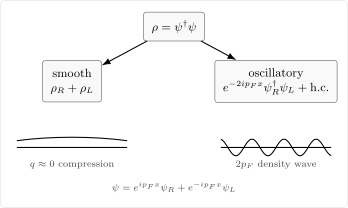
The one-dimensional density contains a smooth component $\rho_R+\rho_L$ and an oscillatory $2p_F$ component. The latter is the field-theory avatar of a charge-density wave.

The same decomposition also explains why one-dimensional interactions are delicate. A short-range microscopic interaction contains Fourier components near $q=0$ and $q=2p_F$. The first gives forward scattering; the second gives backscattering between left and right movers. Both are marginal by power counting in the linearized theory.

The one-dimensional Lindhard function

The free density response is still the particle-hole bubble from the previous page:

$$\chi^R(\omega,q)=\int {dp\over2\pi} {n_p-n_{p+q}\over\omega+i0+\xi_p-\xi_{p+q}}, \qquad n_p=\theta(p_F-|p|).$$

For the static response of the parabolic band, set $\omega=0$. Since

$$\xi_p-\xi_{p+q} =-{q\over m}\left(p+{q\over2}\right),$$

a short calculation gives

$$\boxed{ \chi^R(0,q) =-{m\over\pi q}\log\left|{q+2p_F\over q-2p_F}\right|. }$$

The first check is the long-wavelength limit. Expanding the logarithm at $q\to0$ gives

$$\chi^R(0,q\to0)=-{m\over\pi p_F}=-{1\over\pi v_F}.$$

This is minus the one-dimensional density of states at the Fermi level. That sign agrees with the convention that $U$ is a potential energy.

The second check is the important one: near $q=2p_F$,

$$\chi^R(0,q) \simeq -{1\over2\pi v_F} \log {4p_F\over |q-2p_F|} +\text{regular terms}.$$

The response diverges logarithmically. This is the Peierls singularity.

Here and below, $\Lambda$ denotes a momentum width around each Fermi point and

$$E_c=v_F\Lambda$$

is the corresponding ultraviolet energy of the linearized theory. Keeping these two cutoffs distinct prevents dimensionally inconsistent logarithms.

The dynamic long-wavelength response is also useful. In the linearized theory, the right and left movers give

$$\boxed{ \chi^R_{q\approx0}(\omega,q) ={v_F q^2\over\pi\left[(\omega+i0)^2-v_F^2q^2\right]}. }$$

At $q=0$ and $\omega\neq0$, this vanishes. A spatially uniform, time-dependent potential coupled to total particle number can be removed by a time-dependent phase rotation of $\psi$; it cannot create a density fluctuation. The static limit is different:

$$\lim_{q\to0}\chi^R(0,q)=-{1\over\pi v_F}.$$

This is the same noncommutativity of limits that already appeared in the previous page, now in its sharp one-dimensional form.

The Peierls logarithm from chiral fields

The logarithm at $2p_F$ has a simple field-theory origin. The operator

$$\mathcal O_{2p_F}=\psi_R^\dagger\psi_L$$

annihilates a left mover and creates a right mover. Its susceptibility is a right-left bubble. In Euclidean frequency-momentum variables, its singular part has the form

$$\chi_{2p_F}(i\Omega,Q) =\int {d\omega\,dk\over(2\pi)^2} {1\over i\omega-v_F k} {1\over i(\omega+\Omega)+v_F(k+Q)},$$

where $Q=q-2p_F$ is the deviation from perfect nesting. The poles approach each other when both $\Omega$ and $Q$ are small. Equivalently, after the frequency integral the remaining momentum integral behaves as

$$\int^{\Lambda}{dk\over |k|+\text{infrared cutoff}}.$$

Therefore

$$\boxed{ \chi_{2p_F}(i\Omega,Q) =-{1\over2\pi v_F} \log {E_c\over\sqrt{v_F^2Q^2+\Omega^2}} +\text{regular terms}. }$$

The product of propagators is negative at $Q=\Omega=0$,

$${1\over i\omega-v_Fk}{1\over i\omega+v_Fk} =-{1\over\omega^2+v_F^2k^2},$$

so the response kernel has the same negative sign as the static Lindhard function. Its magnitude grows logarithmically as the energy and momentum deviation from nesting go to zero.

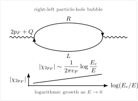
The $2p_F$ density susceptibility is a right-left particle-hole bubble. Perfect nesting leaves an integral $\int dk/|k|$, producing the Peierls logarithm.

There is a complementary position-space way to see the same logarithm. For free chiral fermions in Euclidean spacetime,

$$\langle \psi_R(x,\tau)\psi_R^\dagger(0,0)\rangle \sim {1\over x+i v_F\tau}, \qquad \langle \psi_L(x,\tau)\psi_L^\dagger(0,0)\rangle \sim {1\over x-i v_F\tau}.$$

Thus

$$\langle \mathcal O_{2p_F}(x,\tau)\mathcal O_{2p_F}^\dagger(0,0)\rangle \sim {1\over x^2+v_F^2\tau^2}.$$

Integrating this correlation function over two-dimensional Euclidean spacetime gives

$$\int_a^L {r\,dr\over r^2}\sim \log {L\over a}.$$

So the Peierls logarithm is simply the logarithmic integral of an operator with dimension one in $1+1$ dimensions.

This position-space argument also explains why interactions change exponents in a Luttinger liquid. The free operator $\mathcal O_{2p_F}$ has dimension one, giving a logarithm when integrated over two Euclidean dimensions. Interactions can shift the scaling dimension, turning the logarithm into a power-law enhancement or suppression.

RPA criterion and soft modes

A logarithm in the free susceptibility does not by itself prove that the ground state has ordered. It says that a weak perturbation in the corresponding channel is strongly amplified. A useful diagnostic is the random-phase denominator. For a density-density interaction with Fourier component $V(q)$,

$$\chi_{\rm RPA}(\omega,q) ={\chi_0(\omega,q)\over1-V(q)\chi_0(\omega,q)}.$$

In the static $2p_F$ channel,

$$\chi_0(0,2p_F+Q) \simeq -{1\over2\pi v_F}\log {E_c\over v_F|Q|}.$$

If the effective interaction is attractive in this channel, $V(2p_F)<0$, then the denominator can vanish:

$$1-V(2p_F)\chi_0=0.$$

For weak attraction this occurs at the exponentially small scale

$$E_{\rm P}\sim E_c\exp\left[-{2\pi v_F\over |V(2p_F)|}\right].$$

This is the Peierls scale in its simplest mean-field form. In an electron-phonon system, the same logarithm softens the phonon at wavevector $2p_F$, making a lattice distortion energetically favorable. In a purely electronic model, the same singularity signals a strong charge-density-wave or spin-density-wave tendency, depending on the spin structure of the interaction.

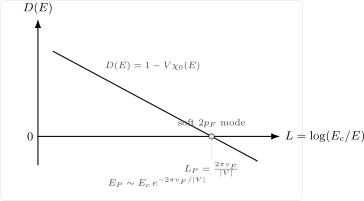
For an attractive nested-channel interaction, $D(E)=1-V\chi_0(E)$ decreases linearly with $L=\log(E_c/E)$. Its zero marks a soft $2p_F$ mode, not merely a large perturbative correction.

This logic is the finite-density cousin of other instabilities. For electric Coulomb repulsion, screening makes long-wavelength potentials less singular. For an attractive long-range force, the sign of the response denominator is reversed and a homogeneous state can become unstable, the many-body analogue of the Jeans instability. The moral is the same: once a response denominator vanishes, the assumed background is no longer the correct saddle point.

RPA is only a channel diagnostic here. In one dimension, vertex corrections in the Peierls and Cooper channels can carry logarithms of the same order as the bubble chain. The controlled infrared description is an RG or bosonized theory; the RPA zero correctly identifies a dangerous channel but does not by itself determine the one-dimensional phase.

Cooper and Peierls channels

The Peierls logarithm is not the only logarithm. The Cooper channel is also logarithmic. A right mover and a left mover with total momentum zero can repeatedly scatter into another pair with total momentum zero. The loop integral has the same radial structure:

$$\Pi_{\rm C}(E) \sim \int_{E<\sqrt{\omega^2+v_F^2k^2}<E_c} {d\omega\,dk\over(2\pi)^2} {1\over \omega^2+v_F^2k^2} ={1\over2\pi v_F}\log {E_c\over E}.$$

In dimensions $d>1$, the Cooper channel is still logarithmic because momenta $\mathbf p$ and $-\mathbf p$ both lie on the Fermi surface. What is special in one dimension is that the particle-hole channel at $2p_F$ is logarithmic too, and the same two Fermi points participate in both channels.

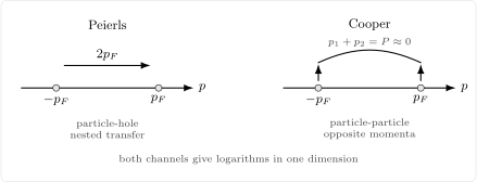
Two logarithmic channels compete in one dimension. The Peierls arrow denotes momentum transfer near $2p_F$; the Cooper arc groups opposite momenta whose sum is near zero.

This competition is why one-dimensional fermions are not well described by a stable Landau Fermi liquid. In a Landau Fermi liquid, quasiparticles remain sharply defined and most interactions are perturbatively harmless at low energy. In one dimension, forward scattering is exactly marginal, while backscattering and pairing channels can produce logarithmic flow. Even when no conventional long-range order forms, the free-fermion exponents are generally replaced by interaction-dependent power laws. The resulting gapless phase is a Luttinger liquid.

A compact way to organize short-range interactions is the $g$-ology notation. For spinless fermions one may write, schematically,

$$H_{\rm int} = g_4(\rho_R^2+\rho_L^2)+g_2\rho_R\rho_L +g_1\psi_R^\dagger\psi_L\psi_L^\dagger\psi_R+\cdots.$$

Here $g_4$ is same-branch forward scattering, $g_2$ is opposite-branch forward scattering, and $g_1$ is backscattering near $2p_F$. For spinful fermions, the charge and spin combinations of these couplings flow differently. On a lattice at commensurate filling, umklapp terms can also become important and open a Mott gap.

For a strictly local spinless interaction, Fermi antisymmetry relates some of these amplitudes and can make a nominal contact term vanish. The labels are independent most transparently for spinful fermions or finite-range interactions. The channel classification, rather than the number of independent bare constants, is what will survive into the RG analysis.

At this stage the important point is not the full $g$-ology phase diagram, but the mechanism: logarithmic susceptibilities turn apparently marginal four-fermion interactions into running couplings. The later bosonization pages will replace these loop warnings by a more complete fixed-point description.

For this reason, the spinless formulas on this page should be treated as kinematic diagnostics, not as the full phase diagram. They identify the dangerous channels; the actual infrared fixed point depends on spin, symmetries, commensurability, and the signs of the marginal couplings.

The detailed solution belongs to later pages, but the warning belongs here: a logarithm is the perturbative announcement that the infrared theory has reorganized itself.

Example: opening a Peierls gap

Suppose an external or self-consistent distortion couples to the $2p_F$ density operator. Write the mean-field Hamiltonian density as

$$\mathcal H_{\rm MF} =-i v_F\psi_R^\dagger\partial_x\psi_R +i v_F\psi_L^\dagger\partial_x\psi_L +\Delta\psi_R^\dagger\psi_L +\Delta^*\psi_L^\dagger\psi_R.$$

In momentum space this is

$$H_{\rm MF}=\int {dk\over2\pi} \begin{pmatrix}\psi_R^\dagger(k)&\psi_L^\dagger(k)\end{pmatrix} \begin{pmatrix} v_F k & \Delta\\ \Delta^* & -v_F k \end{pmatrix} \begin{pmatrix}\psi_R(k)\\ \psi_L(k)\end{pmatrix}.$$

The quasiparticle energies are

$$\boxed{ E_\pm(k)=\pm\sqrt{v_F^2k^2+|\Delta|^2}. }$$

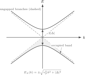
A $2p_F$ distortion mixes right and left movers. The crossing of the two linear branches is avoided, and a gap $2|\Delta|$ opens at the Fermi energy.

The filled negative-energy band lowers the ground-state energy because the states near the crossing move downward. Subtracting the $\Delta=0$ band energy, the singular part of the energy density behaves as

$$\delta\mathcal E_{\rm fermion} \sim -{|\Delta|^2\over2\pi v_F}\log {E_c\over |\Delta|}.$$

A lattice or order-parameter stiffness contributes a positive analytic term, for example $|\Delta|^2/(2\lambda)$. Because the fermionic term contains an extra logarithm, any weak attractive coupling can win at sufficiently low energy in the mean-field treatment. The result is a gap of the same exponential form as the instability scale.

This example is deliberately parallel to the BCS gap mechanism. The algebra differs by channel: BCS pairs particles with opposite momenta, while Peierls pairs a particle and a hole separated by $2p_F$. The shared feature is a logarithmic infrared enhancement.

This distinction matters experimentally and theoretically. A self-consistent Peierls gap breaks translation symmetry through a density modulation; an externally imposed distortion breaks translation explicitly. A BCS gap instead diagnoses pairing and, in a mean-field or higher-dimensional superconducting phase, broken particle-number symmetry. Similar exponentials do not imply identical order parameters.

Summary

In one dimension the Fermi surface consists of two nested points. This makes the density response unusually singular. The exact static free response for a parabolic band is

$$\chi^R(0,q) =-{m\over\pi q}\log\left|{q+2p_F\over q-2p_F}\right|,$$

so the response diverges logarithmically near $q=2p_F$. In the linearized theory, the same logarithm is the susceptibility of the operator

$$\mathcal O_{2p_F}=\psi_R^\dagger\psi_L.$$

The density decomposes as

$$\rho=\rho_R+\rho_L+e^{-2ip_Fx}\mathcal O_{2p_F}+e^{2ip_Fx}\mathcal O_{2p_F}^\dagger,$$

which identifies the oscillatory charge-density-wave channel. An attractive interaction in this channel can drive an RPA denominator to zero and open a Peierls gap. Meanwhile, the Cooper channel is logarithmic as well. The coexistence of these logarithmic channels is the perturbative reason one-dimensional fermions flow away from the naive free Fermi gas and toward Luttinger-liquid, density-wave, superconducting, or gapped behavior depending on symmetries and interactions.

Common pitfalls

Calling the $2p_F$ singularity ultraviolet. It is an infrared effect at a nonzero momentum set by the separation of the Fermi points.

Interchanging static and dynamic response. The functions $\chi^R(0,q)$ and $\chi^R(\omega,0)$ answer different questions. A uniform time-dependent scalar potential is a phase rotation; a static spatial modulation rearranges occupied states.

Equating a divergent bubble with proven long-range order. A logarithm in a susceptibility is a warning, not automatically a proof of order. In strictly one dimension, fluctuations are strong. Depending on the interaction and symmetries, the outcome may be a gap, a density wave, a spin gap, superconducting correlations, or a gapless Luttinger liquid with power-law order. Mean-field language identifies the dangerous channel; it does not replace the infrared solution.

Mixing the Peierls and Cooper channels. The former is particle-hole nesting at momentum transfer near $2p_F$; the latter is particle-particle pairing at total momentum near zero.

Multiplying every spinless result by two. This is safe for free density response, but interactions split into charge and spin channels, and their RG flows are not obtained by a simple degeneracy factor.

Using one symbol for momentum and energy cutoffs. A patch width $\Lambda$ has units of momentum; the linearized energy cutoff is $E_c=v_F\Lambda$. The Peierls and Cooper logarithms must compare quantities with the same units.

Exercises

Exercise 1: Derive the one-dimensional static Lindhard function

Starting from

$$\chi^R(0,q)=\int {dp\over2\pi} {n_p-n_{p+q}\over\xi_p-\xi_{p+q}+i0}, \qquad n_p=\theta(p_F-|p|),$$

with $\xi_p=p^2/(2m)-\mu$, derive

$$\chi^R(0,q) =-{m\over\pi q}\log\left|{q+2p_F\over q-2p_F}\right|.$$

Solution

Write

$$\chi^R(0,q)=\int {dp\over2\pi} {n_p\over\xi_p-\xi_{p+q}} -\int {dp\over2\pi} {n_{p+q}\over\xi_p-\xi_{p+q}}.$$

In the second integral set $p'=p+q$ and then rename $p'\to p$:

$$\chi^R(0,q)=\int_{-p_F}^{p_F}{dp\over2\pi} \left[ {1\over\xi_p-\xi_{p+q}} -{1\over\xi_{p-q}-\xi_p} \right].$$

For the parabolic dispersion,

$$\xi_p-\xi_{p+q}=-{q\over m}\left(p+{q\over2}\right), \qquad \xi_{p-q}-\xi_p=-{q\over m}\left(p-{q\over2}\right).$$

Therefore

$$\chi^R(0,q) =-{m\over2\pi q}\int_{-p_F}^{p_F}dp \left({1\over p+q/2}-{1\over p-q/2}\right).$$

The integral is elementary:

$$\chi^R(0,q) =-{m\over2\pi q} \left[ \log|p+q/2|-\log|p-q/2| \right]_{-p_F}^{p_F}.$$

Evaluating the endpoints gives

$$\chi^R(0,q) =-{m\over\pi q} \log\left|{p_F+q/2\over p_F-q/2}\right| =-{m\over\pi q}\log\left|{q+2p_F\over q-2p_F}\right|.$$

Exercise 2: Separate smooth and oscillatory density components

Show that the one-dimensional density operator decomposes as

$$\rho(x)=\rho_R(x)+\rho_L(x)+e^{-2ip_Fx}\psi_R^\dagger\psi_L+e^{2ip_Fx}\psi_L^\dagger\psi_R.$$

Explain why the last two terms describe a density wave with wavevector $2p_F$.

Solution

Using

$$\psi=e^{ip_Fx}\psi_R+e^{-ip_Fx}\psi_L, \qquad \psi^\dagger=e^{-ip_Fx}\psi_R^\dagger+e^{ip_Fx}\psi_L^\dagger,$$

we get

$$\psi^\dagger\psi =\psi_R^\dagger\psi_R+\psi_L^\dagger\psi_L +e^{-2ip_Fx}\psi_R^\dagger\psi_L +e^{2ip_Fx}\psi_L^\dagger\psi_R.$$

The first two terms vary slowly if $\psi_R$ and $\psi_L$ are slowly varying. The cross terms carry phases $e^{\pm2ip_Fx}$, so their real part oscillates as $\cos(2p_Fx+\varphi)$. They therefore represent a density modulation with wavevector $2p_F$ and wavelength $\pi/p_F$.

Exercise 3: Recover the Peierls logarithm from scaling

Use the scaling form

$$\langle \mathcal O_{2p_F}(x,\tau)\mathcal O_{2p_F}^\dagger(0,0)\rangle \sim {1\over x^2+v_F^2\tau^2}$$

to show that the static $2p_F$ susceptibility is logarithmically divergent.

Solution

The magnitude of the susceptibility is the spacetime integral of the correlation function. Up to normalization and the response-sign convention,

$$|\chi_{2p_F}|\sim \int dx\,d\tau\,{1\over x^2+v_F^2\tau^2}.$$

Set $y=v_F\tau$, so $dx\,d\tau=dx\,dy/v_F$. In polar coordinates in the $(x,y)$ plane,

$$|\chi_{2p_F}|\sim {1\over v_F}\int {r\,dr\,d\theta\over r^2}.$$

With a short-distance cutoff $a$ and long-distance cutoff $L$,

$$|\chi_{2p_F}|\sim {2\pi\over v_F}\int_a^L {dr\over r} \sim {2\pi\over v_F}\log {L\over a}.$$

The precise prefactor depends on the normalization of the chiral propagators, but the logarithm is universal at the free fixed point.

Exercise 4: Find the RPA soft-mode scale

Assume the static $2p_F$ susceptibility has singular part

$$\chi_0(0,2p_F+Q)=-C\log {\Lambda\over |Q|}, \qquad C={1\over2\pi v_F},$$

and that an attractive interaction $V(2p_F)=-|V|$ is treated in RPA:

$$\chi_{\rm RPA}={\chi_0\over1-V\chi_0}.$$

Here $\Lambda$ is a momentum cutoff. Find the momentum scale $Q_*$ at which the denominator vanishes and the corresponding energy $E_*=v_F|Q_*|$.

Solution

The denominator is

$$1-V\chi_0 =1-(-|V|)\left[-C\log {\Lambda\over |Q|}\right] =1-|V|C\log {\Lambda\over |Q|}.$$

The zero occurs when

$$|V|C\log {\Lambda\over |Q_*|}=1.$$

Thus

$$|Q_*|=\Lambda\exp\left[-{1\over |V|C}\right] =\Lambda\exp\left[-{2\pi v_F\over |V|}\right].$$

Multiplying by $v_F$ gives the corresponding energy scale.

$$E_*=v_F\Lambda\exp\left[-{2\pi v_F\over|V|}\right] =E_c\exp\left[-{2\pi v_F\over|V|}\right].$$

Exercise 5: Diagonalize the Peierls mean-field Hamiltonian

Diagonalize the mean-field Hamiltonian matrix

$$h(k)= \begin{pmatrix} v_F k & \Delta\\ \Delta^* & -v_F k \end{pmatrix}$$

and show that a gap $2|\Delta|$ opens at $k=0$.

Solution

The eigenvalues solve

$$\det[h(k)-E]=0.$$

Therefore

$$\det \begin{pmatrix} v_F k-E & \Delta\\ \Delta^* & -v_F k-E \end{pmatrix} =(v_F k-E)(-v_F k-E)-|\Delta|^2=0.$$

This gives

$$E^2-v_F^2k^2-|\Delta|^2=0,$$

so

$$E_\pm(k)=\pm\sqrt{v_F^2k^2+|\Delta|^2}.$$

At $k=0$ the two energies are $\pm|\Delta|$, so the separation between the upper and lower bands is $2|\Delta|$.

References

• F. D. M. Haldane, “Luttinger liquid theory of one-dimensional quantum fluids. I. Properties of the Luttinger model and their extension to the general 1D interacting spinless Fermi gas,” Journal of Physics C: Solid State Physics 14 (1981), 2585–2609.
• R. E. Peierls, Quantum Theory of Solids (Clarendon Press, 1955).
• R. Shankar, “Renormalization-group approach to interacting fermions,” Reviews of Modern Physics 66 (1994), 129–192.
• J. Sólyom, “The Fermi gas model of one-dimensional conductors,” Advances in Physics 28 (1979), 201–303.

Further reading

• T. Giamarchi, Quantum Physics in One Dimension (Oxford University Press, 2004).
• A. O. Gogolin, A. A. Nersesyan, and A. M. Tsvelik, Bosonization and Strongly Correlated Systems (Cambridge University Press, 1998).
• G. Grüner, Density Waves in Solids (Addison–Wesley, 1994).
• A. Zee, Quantum Field Theory in a Nutshell, 2nd ed. (Princeton University Press, 2010).