Running Charge, Screening, and Antiscreening

The previous page computed the one-loop photon vacuum polarization and found that gauge invariance forces the answer into the transverse form

$$\Pi_{\mu\nu}(q)=\left(q^2\delta_{\mu\nu}-q_\mu q_\nu\right)\Pi(q^2).$$

That tensor statement is already a renormalization-group statement in disguise. The coefficient of $F_{\mu\nu}F_{\mu\nu}$ is not just a constant appearing in the microscopic Lagrangian; it is a scale-dependent quantity. The value of the electric charge extracted from a scattering experiment depends on the momentum transfer used to probe the charge.

The physical picture is old and robust: the vacuum behaves like a polarizable medium. A positive test charge attracts virtual negative charge and repels virtual positive charge, so an observer far away sees a smaller net charge than an observer who probes inside the polarization cloud. In QED this is screening. In non-Abelian gauge theory the gauge bosons themselves carry charge, and their spin response can reverse the sign. The result is antiscreening and, in four-dimensional Yang–Mills theory, asymptotic freedom.

Running charge from the transverse kernel

Key normalization. We continue to use the rescaled Euclidean gauge-field normalization

$$\Gamma[A] \supset {1\over4}\int d^4x\,{1\over e^2}F_{\mu\nu}F_{\mu\nu},$$

so positively charged matter has unit charge in $D_\mu=\partial_\mu-iA_\mu$. In this convention matter loops correct $1/e^2$ directly. In canonical normalization, the same physics appears as a photon self-energy proportional to $e^2$.

For a Euclidean momentum transfer $q$, the running coupling is defined by the transverse two-point kernel,

$$\Gamma^{(2)}[A] ={1\over2}\int_q A_\mu(-q) \left(q^2\delta_{\mu\nu}-q_\mu q_\nu\right) {1\over e^2(q)}A_\nu(q)+\cdots.$$

Sign check: momentum space versus distance space

For QED matter, $b_{\rm QED}>0$ and

$${1\over e^2(q)}={1\over e^2(\mu)}+{b_{\rm QED}\over16\pi^2}\log{\mu^2\over q^2}.$$

So lowering the momentum transfer below $\mu$ increases $1/e^2(q)$ and decreases $e^2(q)$. Since a distance $r$ probes roughly $q\sim1/r$, large distances see a smaller electric charge. This is the easiest way to keep the signs straight: QED charge grows with momentum and shrinks with distance.

For $N_f$ Dirac fermions and $N_s$ complex scalars of unit Abelian charge, the one-loop logarithm from the previous page can be summarized as

$${1\over e^2(q)} ={1\over e_0^2} +{b_{\rm QED}\over16\pi^2}\log{\Lambda^2\over q^2} +\text{finite local terms},$$

with

$$\boxed{ b_{\rm QED}={4\over3}N_f+{1\over3}N_s. }$$

The cutoff $\Lambda$ is only a temporary way of displaying the logarithm. Define the renormalized charge at a reference scale $\mu$ by

$${1\over e^2(\mu)} ={1\over e_0^2} +{b_{\rm QED}\over16\pi^2}\log{\Lambda^2\over\mu^2} +\text{the same finite convention}.$$

Subtracting the two equations eliminates the bare charge and the cutoff:

$$\boxed{ {1\over e^2(q)} ={1\over e^2(\mu)} +{b_{\rm QED}\over16\pi^2}\log{\mu^2\over q^2} +\text{higher-loop terms}. }$$

Inverting this relation perturbatively gives

$$e^2(q)=e^2(\mu) \left[ 1-{b_{\rm QED}e^2(\mu)\over16\pi^2}\log{\mu^2\over q^2} +O(e^4) \right].$$

Thus, if $q<\mu$, the logarithm is positive and $e^2(q)<e^2(\mu)$. The effective electric charge is smaller at longer distances. If $q>\mu$, the logarithm is negative and $e^2(q)>e^2(\mu)$. Short-distance probes see more of the unscreened charge.

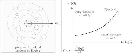
QED screening. A positive external charge polarizes the vacuum: negative induced charge is pulled inward and positive induced charge is pushed outward. A long-distance Gaussian surface encloses a reduced effective charge, while a short-distance probe sees closer to the bare charge.

The beta function follows by differentiating at fixed bare charge:

$$\beta(e)=\mu{de\over d\mu}.$$

Since

$${d\over d\log\mu}{1\over e^2(\mu)} =-{2b_{\rm QED}\over16\pi^2},$$

and

$${d\over d\log\mu}{1\over e^2} =-{2\over e^3}\beta(e),$$

we obtain

$$\boxed{ \beta_{\rm QED}(e) ={b_{\rm QED}\over16\pi^2}e^3+O(e^5). }$$

The positive sign is the algebraic version of screening.

Static potential and the meaning of a measured charge

A useful operational definition of the electric charge is the strength of the Coulomb interaction at momentum transfer $\mathbf q$. In the static limit, integrating out the photon gives

$$V(\mathbf q)={e^2(|\mathbf q|)\over \mathbf q^2}$$

up to convention-dependent factors such as the charges of the external sources. In position space, a renormalization-group-improved estimate is

$$V(r)\simeq {e^2(1/r)\over4\pi r}.$$

This is not an exact Fourier transform of the logarithmic expression, but it captures the scale choice: a separation $r$ mostly probes momenta $q\sim 1/r$.

For QED matter with $b_{\rm QED}>0$,

$$e^2(1/r)$$

decreases as $r$ increases. The long-distance electric field is weaker than it would be in the absence of vacuum polarization. In a medium this would be expressed by a dielectric constant $\epsilon>1$. In the field-theory normalization used here, the analog of the dielectric constant is the coefficient $1/e^2(q)$ multiplying $F^2$: it grows in the infrared.

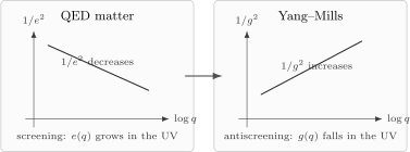
At one loop, QED matter screens charge: the inverse Abelian coupling decreases toward short distances. Pure Yang–Mills theory antiscreens: the inverse non-Abelian coupling increases toward short distances.

The perturbative QED solution can be written as

$${1\over e^2(\mu)} ={1\over e^2(\mu_0)} -{b_{\rm QED}\over8\pi^2}\log{\mu\over\mu_0}.$$

If this one-loop equation is extrapolated far enough into the ultraviolet, the denominator reaches zero at

$$\mu_L =\mu_0\exp\left({8\pi^2\over b_{\rm QED}e^2(\mu_0)}\right).$$

This is the Landau pole of perturbative QED. It should not be overinterpreted as a directly observable catastrophe in real-world QED; before arbitrarily high energies are reached, QED is embedded in the electroweak theory, and in any case a perturbative extrapolation beyond its own singularity is not evidence. The reliable lesson is more modest and more important: pure QED is not asymptotically free.

Closed worldlines and vacuum polarization

The loop correction to $F^2$ has a path-integral representation. Consider one charged complex scalar with Euclidean operator $L_A=-D^2+m^2$, $m^2>0$, and fixed boundary conditions. Begin with positive finite mode matrices for $L_A$ and $L_0=-\partial^2+m^2$, using a common cutoff independent of $m^2$. The propagator can be written in proper time as

$$G_A(x,x')= \int_0^\infty dT\,e^{-m^2T}K_A(x,x';T),$$

where the heat kernel is a sum over paths,

$$K_A(x,x';T)= \int_{x(0)=x'}^{x(T)=x}\mathcal D x(\tau)\, \exp\left[ -{1\over4}\int_0^T d\tau\,\dot x^2 +i\int_0^T d\tau\,\dot x^\mu A_\mu(x(\tau)) \right].$$

The Gaussian scalar integral gives a determinant. Its contribution to the effective action, with the zero-field value subtracted, is

$$\begin{aligned} \Gamma_s[A]-\Gamma_s[0] &=\operatorname{Tr}\log L_A-\operatorname{Tr}\log L_0,\\ \frac{\partial}{\partial m^2}\bigl(\Gamma_s[A]-\Gamma_s[0]\bigr) &=\operatorname{Tr}\bigl(L_A^{-1}-L_0^{-1}\bigr). \end{aligned}$$

The second line is a difference of propagator traces; the effective action itself contains the logarithms. Integrating the mass derivative produces the extra $1/T$ in the proper-time measure. The heat-kernel trace sets the final point equal to the initial point and integrates that base point, so the paths close. For the continuum heat kernel, introduce a proper-time cutoff $\epsilon>0$ and write the regulated action difference as

$$\Delta\Gamma_{s,\epsilon}[A] =-\int_\epsilon^\infty {dT\over T}\,e^{-m^2T} \int_{x(T)=x(0)}\mathcal D x\,e^{-\frac14\int_0^T\dot x^2d\tau} \left(e^{i\oint A_\mu dx^\mu}-1\right).$$

At finite $\epsilon$, the mass derivative of this expression is $\operatorname{Tr}(e^{-\epsilon L_A}L_A^{-1}-e^{-\epsilon L_0}L_0^{-1})$, the correspondingly regulated propagator trace. The uncut identities above are recovered when the limit exists. In four continuum dimensions, subtracting the $A=0$ term removes the field-independent contribution but leaves the $F^2$ ultraviolet divergence; a Maxwell counterterm is still needed before removing the cutoff. The determinant, mass derivative and closed-loop interpretation are developed in Schwartz 2014, §§ 33.2.3–33.3, pp. 710–712. Here the Euclidean complex-scalar Gaussian gives $+\operatorname{Tr}\log L_A$; the cited Lorentzian expression carries the corresponding factors of $i$.

The factor

$$W[x]=e^{i\oint A_\mu dx^\mu}$$

is a Wilson loop around the virtual particle trajectory. For a small loop of size $\ell$ in a smooth, approximately constant field,

$$\oint A_\mu dx^\mu ={1\over2}F_{\mu\nu}\delta\sigma^{\mu\nu} +O(\ell^3\partial F),$$

where

$$\delta\sigma^{\mu\nu} ={1\over2}\oint\bigl(x^\mu dx^\nu-x^\nu dx^\mu\bigr)$$

is the oriented area tensor of the loop, and both ordered values of each antisymmetric index pair are summed. For a counterclockwise rectangle of area $S$ in the 12-plane, $\delta\sigma^{12}=S$ and $\delta\sigma^{21}=-S$. With $F_{12}=B=-F_{21}$, the contraction is $\tfrac12(BS+(-B)(-S))=BS$, as required by Stokes’ theorem. Reversing the loop reverses the flux. The small-loop holonomy calculation and Schwartz 2014, § 25.5, pp. 504–505 give the corresponding oriented plaquette expansion. Expanding the Wilson factor with this area convention gives

$$\left\langle e^{i\oint A\cdot dx}\right\rangle =1-{1\over8}F_{\mu\nu}F_{\rho\sigma} \left\langle\delta\sigma^{\mu\nu}\delta\sigma^{\rho\sigma}\right\rangle+\cdots.$$

The linear term vanishes after averaging over loop orientations. The quadratic term is local and proportional to $F_{\mu\nu}F_{\mu\nu}$. This is the worldline version of vacuum polarization: small closed charged paths sample the flux of the background field, and their accumulated phases renormalize the Maxwell action.

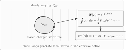
A charged virtual particle loop carries the Wilson phase $e^{i\oint A\cdot dx}$. For a small loop, the summed contraction is $\tfrac12F_{\mu\nu}\delta\sigma^{\mu\nu}$, with the area tensor defined above; it equals $BS$ for a planar loop in a constant magnetic field. Orientation averaging produces local terms such as $F_{\mu\nu}F_{\mu\nu}$ in the effective action. The diagram is schematic.

This picture is especially useful because it separates two effects that are often hidden inside Feynman-parameter integrals. First, there is an orbital response: charged particles moving in loops respond to the magnetic flux through the loop. Second, if the particle has spin, there is a spin response: the spin couples directly to the background field.

Classical gas, quantum loops, and magnetic susceptibility

The orbital response is genuinely quantum. Consider a classical nonrelativistic gas of particles in a static vector potential,

$$H(\mathbf p,\mathbf x)={1\over2m}\left(\mathbf p-e\mathbf A(\mathbf x)\right)^2.$$

The classical partition function is

$$Z_{\rm cl}[A]=\int d^3x\,d^3p\, \exp\left[-\beta {\left(\mathbf p-e\mathbf A(\mathbf x)\right)^2\over2m}\right].$$

At each fixed $\mathbf x$, shift the integration variable

$$\mathbf p'=\mathbf p-e\mathbf A(\mathbf x).$$

The measure is unchanged, so

$$Z_{\rm cl}[A]=Z_{\rm cl}[0].$$

A classical gas has no equilibrium orbital magnetic susceptibility. This is the Bohr–van Leeuwen theorem in its simplest form.

Quantum mechanically the same shift is not harmless, because the kinetic momenta

$$\boldsymbol\Pi=\mathbf p-e\mathbf A(\mathbf x)$$

fail to commute:

$$[\Pi_i,\Pi_j]=ieF_{ij}.$$

Equivalently, the trace

$$Z_{\rm qm}[A]=\operatorname{Tr}e^{-\beta H(\mathbf p-e\mathbf A,\mathbf x)}$$

has an imaginary-time path-integral representation with closed paths weighted by

$$\exp\left(i e\oint \mathbf A\cdot d\mathbf x\right).$$

The magnetic field cannot be removed from the trace by a classical change of variables. Landau levels are precisely the quantum memory of the noncommuting kinetic momenta.

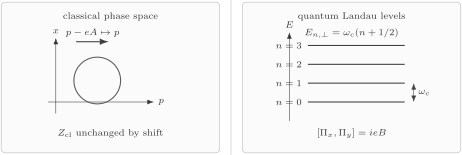
Classically, the vector potential can be removed from the phase-space integral by shifting momentum. Quantum mechanically, covariant momenta do not commute in a magnetic field, and the trace remembers the flux through closed paths. Landau levels are the resulting orbital response.

For a free three-dimensional degenerate gas with isotropic parabolic dispersion $E=\mathbf p^2/(2m)$ and spin gyromagnetic factor $g=2$, the smooth weak-field continuum response separates into orbital Landau diamagnetism and spin Pauli paramagnetism. In this model,

$$\chi_{\rm Landau}=-{1\over3}\chi_{\rm Pauli},$$

so the spin response is larger. Suppressing the spin coupling within the same free parabolic-dispersion model leaves the diamagnetic orbital response. The ratio refers to the smooth susceptibility, with the weak-field limit taken before the zero-temperature limit; it is not a general statement about interacting electrons, arbitrary bands or resolved quantum oscillations. Tong 2012, §§ 3.6.6–3.6.7 derives the two responses in this free-gas setting. The QFT beta function is not this susceptibility, but the comparison illustrates how orbital and spin couplings can contribute with competing signs to a gauge-field effective action.

Antiscreening in Yang–Mills theory

In Abelian gauge theory, photons do not carry electric charge. The vacuum polarization responsible for charge running comes from charged matter. In Yang–Mills theory, the gauge bosons themselves carry the charge of the gauge group. A color field therefore polarizes not only matter, but also the gauge field.

For a pure $SU(N)$ gauge theory, the one-loop beta function is

$$\boxed{ \beta_{\rm YM}(g) =-{g^3\over16\pi^2}{11\over3}C_A+O(g^5), \qquad C_A=N\ \text{for }SU(N). }$$

With $N_f$ Dirac fermions in a representation $R$, this becomes

$$\boxed{ \beta(g) =-{g^3\over16\pi^2} \left({11\over3}C_A-{4\over3}T_RN_f\right)+O(g^5), }$$

where $T_R$ is defined by

$$\operatorname{tr}_R(T^aT^b)=T_R\delta^{ab}.$$

The matter term has the same sign as QED screening. The gauge-boson term has the opposite sign and is larger in pure Yang–Mills theory. For $SU(N)$ with fundamental Dirac fermions, $T_R=1/2$, so asymptotic freedom requires

$$N_f<{11\over2}N.$$

This inequality is not the whole story of confinement or chiral symmetry breaking, but it is the perturbative condition that the ultraviolet fixed point at $g=0$ is attractive.

Integrating the pure Yang–Mills equation gives

$${1\over g^2(q)} ={1\over g^2(\mu)}+{b_0\over8\pi^2}\log{q\over\mu}, \qquad b_0={11\over3}C_A.$$

Thus $g(q)$ decreases at large $q$ and grows at small $q$. The ultraviolet theory becomes weakly coupled, while the infrared theory becomes strongly coupled. The RG-invariant scale is

$$\Lambda_{\rm YM} =\mu\exp\left[-{8\pi^2\over b_0g^2(\mu)}\right].$$

This is dimensional transmutation: a dimensionless coupling has been traded for a physical scale.

Why does the sign reverse? In a background-field calculation, the quadratic operator for gauge fluctuations schematically contains

$$\Delta_{\mu\nu}^{ab} =-(D^2)^{ab}\delta_{\mu\nu} -2f^{acb}F^c_{\mu\nu} +\text{gauge-fixing terms}.$$

The covariant Laplacian $-D^2$ is the orbital part. It behaves like the charged-particle orbital response and tends to screen. The term proportional to $F_{\mu\nu}$ is the spin coupling of a vector particle with gyromagnetic ratio $2$. It is paramagnetic, and for non-Abelian gauge bosons it dominates. Ghosts remove unphysical polarizations and are essential for the precise coefficient, but the physical slogan survives:

$$\text{orbital screening} \quad \text{is beaten by} \quad \text{spin-one paramagnetism}.$$

The word “antiscreening” should not be taken too literally as a classical dielectric model. Non-Abelian charge is not a gauge-invariant scalar density that one can surround with a transparent material. The reliable statement is operational and gauge invariant: the strength of interactions at short distances decreases according to the negative beta function, while the long-distance theory becomes strongly coupled.

Thresholds and effective theories

Running is produced by fluctuations that are active at the scale being probed. A charged particle of mass $m$ contributes to the logarithm when

$$q\gg m,$$

but for

$$q\ll m$$

its contribution becomes local:

$$\Pi(q^2)=\Pi(0)+O(q^2/m^2).$$

The constant $\Pi(0)$ is absorbed into the low-energy value of $1/e^2$, while the $q^2/m^2$ terms become higher-derivative operators such as

$${1\over m^2}(\partial_\rho F_{\mu\nu})(\partial_\rho F_{\mu\nu}).$$

For the momentum-defined charge used here, the heavy contribution to low-energy running is suppressed by $q^2/m^2$. In a matched low-energy EFT, the heavy field is absent from the beta function of the remaining fields, but leaves threshold corrections to the couplings and higher-dimension operators. This is not automatic in a full-theory mass-independent scheme such as $\overline{\mathrm{MS}}$: its beta function retains the heavy field until one changes theory and matches. The momentum-subtraction and minimal-subtraction comparison shows the distinction explicitly.

The same principle is used in QCD when quarks are integrated out across mass thresholds. The beta-function coefficient changes, while physical amplitudes remain continuous after matching. In practice one chooses a matching scale $\mu\sim m$ and relates the couplings just above and just below the threshold,

$$g_{\rm above}(\mu)=g_{\rm below}(\mu)+\text{finite matching correction},$$

then runs with the appropriate beta function on each side. The split into “matching” and “running” is conventional, but their combination is physical.

Summary

The running charge is the coefficient of the transverse gauge-field two-point function. In the rescaled Abelian normalization,

$${1\over e^2(q)} ={1\over e^2(\mu)} +{b_{\rm QED}\over16\pi^2}\log{\mu^2\over q^2}, \qquad b_{\rm QED}={4\over3}N_f+{1\over3}N_s.$$

The positive QED beta function

$$\beta(e)={b_{\rm QED}\over16\pi^2}e^3+O(e^5)$$

means that electric charge is screened at long distances and grows toward short distances. If extrapolated within perturbation theory, this produces a Landau pole.

A worldline representation turns vacuum polarization into the phase accumulated by closed charged paths,

$$e^{i\oint A\cdot dx},$$

whose small-loop expansion generates local terms such as $F^2$. This worldline picture explains why background-field response is local at short proper time, but the sign of the beta function still depends on spin, statistics, and gauge constraints. The magnetic analogy separates orbital diamagnetism from spin paramagnetism. In Yang–Mills theory, spin-one gauge boson paramagnetism dominates the orbital screening contribution. The one-loop beta function becomes negative,

$$\beta(g)=-{g^3\over16\pi^2}{11\over3}C_A+\cdots,$$

so the coupling decreases at short distances and grows in the infrared. This is antiscreening and asymptotic freedom.

Common pitfalls

Confusing the bare and measured charges. The measured charge is specified at a scale. The bare charge $e_0$ is a regulator-dependent parameter used to hold physical quantities fixed as the cutoff changes.

Overinterpreting the Landau pole. It is a warning about ultraviolet extrapolation beyond perturbation theory and the effective theory, not a measured singularity in an experiment.

Taking the dielectric analogy literally in Yang–Mills theory. Non-Abelian color density is not an ordinary gauge-invariant dielectric cloud. The clean statement is the sign of a gauge-invariant beta function or the scale dependence of physical short-distance amplitudes.

Forgetting the threshold prescription. Heavy contributions to the momentum-defined low-energy running are power suppressed. A mass-independent full-theory beta function does not switch them off automatically; match to the lower-field EFT, retaining its threshold corrections and higher-dimension operators.

Applying the classical momentum shift to the quantum trace. The kinetic momenta fail to commute, and closed quantum paths remember the magnetic flux.

Exercises

Exercise 1 — The running-charge beta function

Starting from

$${1\over e^2(q)}={1\over e^2(\mu)}+{b\over16\pi^2}\log{\mu^2\over q^2},$$

derive the one-loop beta function for $e(\mu)$.

Solution

Set $q$ equal to a fixed physical momentum and require that the left-hand side is independent of the arbitrary reference scale $\mu$. Equivalently, differentiate the renormalized relation at fixed bare parameters:

$${d\over d\log\mu}{1\over e^2(\mu)}=-{2b\over16\pi^2}.$$

But

$${d\over d\log\mu}{1\over e^2} =-{2\over e^3}{de\over d\log\mu} =-{2\beta(e)\over e^3}.$$

Therefore

$$-{2\beta(e)\over e^3}=-{2b\over16\pi^2},$$

so

$$\boxed{\beta(e)={b\over16\pi^2}e^3.}$$

Exercise 2 — The QED Landau pole

Solve the one-loop QED beta function

$${de\over d\log\mu}={b\over16\pi^2}e^3, \qquad b>0,$$

and find the scale at which the perturbative solution has a Landau pole.

Solution

It is easiest to differentiate $1/e^2$:

$${d\over d\log\mu}{1\over e^2} =-{2\over e^3}{de\over d\log\mu} =-{2b\over16\pi^2} =-{b\over8\pi^2}.$$

Integrating from $\mu_0$ to $\mu$ gives

$${1\over e^2(\mu)} ={1\over e^2(\mu_0)}-{b\over8\pi^2}\log{\mu\over\mu_0}.$$

The perturbative solution becomes singular when the right-hand side vanishes:

$$0={1\over e^2(\mu_0)}-{b\over8\pi^2}\log{\mu_L\over\mu_0}.$$

Thus

$$\boxed{ \mu_L=\mu_0\exp\left({8\pi^2\over b e^2(\mu_0)}\right). }$$

Exercise 3 — The Bohr–van Leeuwen shift

Show that the classical partition function

$$Z_{\rm cl}[A]=\int d^3x\,d^3p\, \exp\left[-\beta {\left(\mathbf p-e\mathbf A(\mathbf x)\right)^2\over2m}\right]$$

is independent of the static vector potential $\mathbf A(\mathbf x)$, assuming the momentum integration is over all $\mathbb R^3$.

Solution

For fixed $\mathbf x$, define

$$\mathbf p'=\mathbf p-e\mathbf A(\mathbf x).$$

Since this is a translation in momentum space,

$$d^3p'=d^3p.$$

The momentum domain is all of $\mathbb R^3$, so it is unchanged by the shift. Therefore

$$Z_{\rm cl}[A] =\int d^3x\,d^3p'\, \exp\left[-\beta {\mathbf p'^2\over2m}\right] =Z_{\rm cl}[0].$$

The absence of classical orbital magnetic susceptibility is a classical phase-space statement. It fails quantum mechanically because the components of $\mathbf p-e\mathbf A$ do not commute when $\mathbf B\ne0$.

Exercise 4 — The RG-invariant Yang–Mills scale

For pure Yang–Mills theory with

$$\beta(g)=-{b_0\over16\pi^2}g^3, \qquad b_0>0,$$

show that

$$\Lambda=\mu\exp\left[-{8\pi^2\over b_0g^2(\mu)}\right]$$

is independent of $\mu$ at one loop.

Solution

First compute

$${d\over d\log\mu}{1\over g^2} =-{2\over g^3}\beta(g) ={2b_0\over16\pi^2} ={b_0\over8\pi^2}.$$

Now take the logarithm of $\Lambda$:

$$\log\Lambda=\log\mu-{8\pi^2\over b_0g^2(\mu)}.$$

Differentiating gives

$${d\log\Lambda\over d\log\mu} =1-{8\pi^2\over b_0}{d\over d\log\mu}{1\over g^2(\mu)} =1-{8\pi^2\over b_0}{b_0\over8\pi^2} =0.$$

Thus $\Lambda$ is RG invariant at one loop. It is the dynamically generated Yang–Mills scale.

Exercise 5 — Decoupling below a mass threshold

A particle of mass $m$ contributes to a vacuum polarization function of the schematic form

$$\Pi(q^2)=c\log{\Lambda^2\over m^2+x(1-x)q^2}$$

inside a Feynman-parameter integral. Explain why its contribution to the momentum-defined running is power suppressed at $q\ll m$, and distinguish this statement from running in a full-theory mass-independent scheme.

Solution

For $q\ll m$,

$$\log{\Lambda^2\over m^2+x(1-x)q^2} =\log{\Lambda^2\over m^2} -\log\left(1+{x(1-x)q^2\over m^2}\right).$$

Expanding the second logarithm gives

$$\log{\Lambda^2\over m^2+x(1-x)q^2} =\log{\Lambda^2\over m^2} -{x(1-x)q^2\over m^2}+O(q^4/m^4).$$

The first term is independent of $q$ and can be absorbed into the low-energy definition of the gauge coupling. The remaining terms are analytic in $q^2/m^2$ and correspond to local higher-derivative operators. In particular, $q\,d\Pi/dq=O(q^2/m^2)$, so the heavy contribution to this momentum-defined running is suppressed rather than identically zero at finite $q/m$. In a mass-independent full-theory scheme, the heavy field can still contribute to the beta function below its mass. Matching to an EFT without that field transfers its effects into threshold corrections and the higher-dimension operators instead.

References

• Schwartz, Matthew D. Quantum Field Theory and the Standard Model. Cambridge University Press, 2014. DOI.
• Tong, David. Statistical Physics. University of Cambridge lecture notes, 2012, §§ 3.6.6–3.6.7. Online text.

Further reading

• Polyakov, Alexander M. Gauge Fields and Strings. Harwood Academic Publishers, 1987, chapter 2.
• Srednicki, Mark. Quantum Field Theory. Cambridge University Press, 2007, sections 66 and 73.
• Weinberg, Steven. The Quantum Theory of Fields, Volume II: Modern Applications. Cambridge University Press, 1996, chapter 18.
• Zee, A. Quantum Field Theory in a Nutshell. 2nd ed. Princeton University Press, 2010, parts III and VII.
• Zinn-Justin, Jean. Quantum Field Theory and Critical Phenomena. 4th ed. Oxford University Press, 2002, chapters 8–13 and 20–26.