

Decoupling Theorems and Threshold Corrections
Heavy particles decouple when low-energy light-field observables can be reproduced by shifting the light theory’s relevant and marginal parameters and adding a local tower suppressed by powers of the heavy mass. The statement is conditional: the external invariants and light masses must be small compared with a mass that remains large in the limit, the couplings must obey a uniform counting, and symmetry or anomaly information must survive the field removal. In a mass-independent scheme, decoupling is implemented by matching to a new EFT; it does not occur automatically in the beta function.
Required background. Matching Conditions Beyond Tree Level supplies renormalized hard matching. Scheme Transformations and RG Invariants supplies finite coupling maps and scale-invariant predictions. Helpful background. Interacting Fields, Asymptotic Observables, and Effective Descriptions clarifies why the fields and parameters used in two descriptions need not be identical observables.
The conditional decoupling statement
Section titled “The conditional decoupling statement”Let be a heavy mass and let bound every external invariant and light mass relevant to a renormalized light-field matching object. Perturbative decoupling asserts that, for and away from heavy thresholds, one can choose light-field and parameter maps such that
through a declared order . The first line contains unsuppressed threshold shifts of masses, couplings, vacuum terms, and field normalizations. The second contains local higher-dimensional operators. Logs of may occur in either part and are controlled by matching and running.
The theorem requires, in the form used here:
- renormalized external momenta and light masses uniformly below the first omitted heavy singularity;
- a heavy eigenvalue that stays of order as the low-energy limit is taken;
- interactions whose scaling with has been declared and does not invalidate the inverse-mass expansion;
- a local ultraviolet theory and a complete low-energy operator set compatible with its linearly or nonlinearly realized symmetries;
- no heavy external state, resonant kinematics, or unresolved nearly degenerate threshold in the observable; and
- field, gauge, measure, and anomaly terms sufficient to reproduce the light-sector Ward identities.
Under these hypotheses, heavy effects are absorbed into renormalized light parameters or suppressed by inverse powers of . Appelquist and Carazzone establish the perturbative infrared theorem and its assumptions in Appelquist and Carazzone 1975, pp. 2856–2861. The conclusion is about low-energy predictions after parameter matching, not about every heavy-loop contribution vanishing term by term.
Automatic and explicit decoupling schemes
Section titled “Automatic and explicit decoupling schemes”For a Dirac fermion of electric charge and mass , a Euclidean momentum-subtraction scheme gives the one-loop contribution
Its limiting behaviors are
The mass-dependent beta function therefore suppresses the heavy fermion smoothly at low subtraction momentum. In modified minimal subtraction, the same fermion contributes at every because only the ultraviolet pole is subtracted. This is not a physical failure of decoupling; it means the active field content must be changed explicitly and the two renormalized couplings matched. Manohar derives both scheme descriptions in Manohar 2020, § 7, pp. 58–61, Open PDF.
The figure shows the resulting organization. RG evolution never crosses a threshold without a matching map, and every matching step passes through a decoupling-hypothesis check.
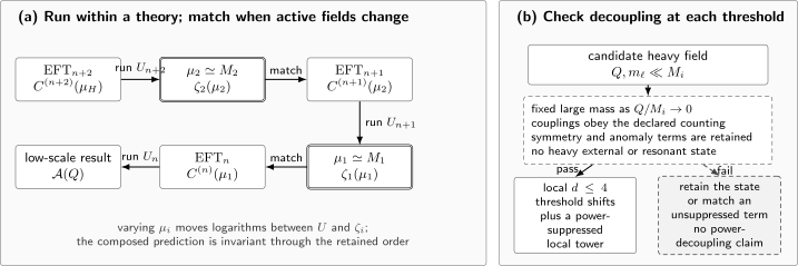
Sequential threshold evolution is an alternation, not one continuous beta function. Panel (a) evolves coefficients with , matches with near , evolves with , matches with near , and finally evolves to the observable scale; dependence on the arbitrary matching scales cancels through the retained order. Panel (b) checks the hierarchy, heavy-mass limit, coupling counting, symmetry and anomaly terms, and external kinematics. Passing gives shifts of operators with dimension at most four plus an inverse-mass-suppressed local tower; failure requires retaining the state or matching an unsuppressed effect. The diagram is schematic and not to scale.
A charged-fermion threshold
Section titled “A charged-fermion threshold”In modified minimal subtraction, the heavy contribution to the renormalized transverse vacuum polarization is
For ,
The constant term is absorbed into the gauge kinetic normalization. Restoring a canonical photon field gives the one-loop threshold relation
or, with ,
At , at this loop order in this scheme. Continuity at the nominal threshold is not a general theorem: finite constants appear at higher loops and in other subtraction conventions. The term instead produces the local operator
up to basis transformations. The first term shifts a marginal parameter without power suppression; the second is a genuinely power-suppressed observable correction. Both are decoupling effects.
Matching-scale independence
Section titled “Matching-scale independence”Write the one-loop Abelian running as
Starting at and ending at , running to an arbitrary matching scale , applying the threshold relation, and running onward gives
Differentiating with respect to the arbitrary matching point yields
Thus the threshold logarithm is fixed by the difference of beta functions. Omitting it leaves an unphysical matching-scale dependence.
For a numerical check, take one unit-charged light fermion, one unit-charged heavy fermion, , and evaluate at .
| High-theory running | Threshold logarithm | Low-theory running | ||
|---|---|---|---|---|
| 0.5 | Included | Included | Included | 129.465871198 |
| 1.0 | Included | 0 | Included | 129.465871198 |
| 2.0 | Included | Included | Included | 129.465871198 |
The equality is exact at the displayed one-loop accuracy. At finite perturbative order, a residual variation of the combined result estimates only missing higher matching and running orders if all other inputs are held fixed. A reproducible calculation can be used to perform this variation.
What can survive the heavy limit
Section titled “What can survive the heavy limit”Decoupling permits several effects that are not visibly suppressed in a Lagrangian coefficient.
- Vacuum energy and scalar masses can receive terms proportional to and . These renormalize relevant operators; their sensitivity is a naturalness question, not by itself a contradiction of decoupling.
- Marginal couplings and field normalizations receive constants and threshold terms. Predictions become power suppressed only after low-energy inputs are fixed consistently.
- An anomaly carried by removed fermions can remain through a Wess–Zumino term or another unsuppressed functional contribution needed to preserve the low-energy symmetry statement.
- If a heavy mass arises from a low-energy order parameter while its coupling grows as , the nominal factors can be cancelled by couplings. The limit then violates the bounded-coupling hypothesis.
- Mixing angles, near-degenerate levels, and resonant external kinematics can make the inverse-mass expansion nonuniform.
These are assumption failures or unsuppressed threshold maps, not licenses to discard matching. Nondecoupling Effects and Matching Validation develops the diagnostic classification.
Matching validation record
Section titled “Matching validation record”The threshold relation is portable only with the active fields, mass definition, charge normalization, subtraction convention, matching scale, and validation observable declared. The chapter’s shared record applies unchanged:
| Record | Declare before matching | Closure check |
|---|---|---|
| Matching object and external data | Amplitude, form factor, Green function, background vertex or functional action; external species, polarizations, momenta and projections | The chosen objects span every coefficient combination claimed |
| Kinematics and retained order | On- or off-shell conditions, exceptional limits, expansion variables, inverse-mass order and loop order | Full and EFT expressions are expanded in the same variables and compared through the same order |
| Fields and normalization | Field coordinates, kinetic normalization, masses, LSZ residues and finite field maps | Two-point functions and external residues agree, or an explicit field transformation relates them |
| Gauge and auxiliary sectors | Quantum and background gauge fixing, ghosts, BRST-exact sectors and anomaly assumptions | Gauge-parameter or auxiliary-sector dependence cancels in the final observable |
| Operator basis and redundancies | Generating or reduced basis, integration-by-parts, equation-of-motion, evanescent and contact sectors | A complete map to the target basis reproduces the same amplitudes or invariant correlators |
| Ultraviolet scheme and matching scale | Regulator, subtraction convention, finite counterterms and | Scheme and dependence cancels against coefficient running and matrix elements through the retained order |
| Infrared prescription | Light masses or virtualities, infrared regulator, overlap or zero-bin subtraction and order of limits | Every common infrared pole and logarithm cancels in full minus EFT before a hard coefficient is read off |
| Threshold and decoupling assumptions | Active fields, heavy-mass origin, coupling scaling, threshold order and hierarchy among heavy scales | Sequential and one-step organizations agree to the claimed order where both are valid |
| Observable closure and uncertainty | Validation observable, input parameters, truncation estimate, numerical tolerance and fit covariance | Independent observables agree within the decomposed uncertainty and show the expected residual scaling |
Common pitfalls
Section titled “Common pitfalls”Heavy fields appear in an MS beta function below their mass, so decoupling failed. A mass-independent beta function does not know when the active field content should change. Match to the lower-field EFT and run with its beta function.
Decoupling means every threshold correction vanishes as . Relevant and marginal parameters can receive unsuppressed shifts. Decoupling concerns low-energy predictions after those parameters are matched.
Coupling continuity is physical. Equality at happens in the one-loop QED example’s chosen scheme. Finite scheme or higher-loop terms can make the parameter discontinuous while observables remain continuous.
A large mass is sufficient. The way the mass and couplings scale, the external kinematics, anomalies, mixing, and the operator content are also hypotheses. Check them before invoking power suppression.
Exercises
Section titled “Exercises”Use and to derive both limits of .
Solution
For , the ratio in the integrand approaches one, so . For , expand the ratio as ; the remaining integral is , giving .
Differentiate the composed inverse-coupling expression with respect to and explain what a nonzero answer would diagnose.
Solution
The derivative is because . A nonzero result at the retained order means the threshold logarithm, one of the beta functions, or the active-field assignment is inconsistent. A remainder beginning at the next loop order is expected in a truncated calculation.
References
Section titled “References”- Appelquist, Thomas, and J. Carazzone. “Infrared Singularities and Massive Fields.” Physical Review D 11, no. 10 (1975): 2856–2861. DOI
- Manohar, Aneesh V. “Introduction to Effective Field Theories.” In Effective Field Theory in Particle Physics and Cosmology: Lecture Notes of the Les Houches Summer School, Volume 108, edited by Sacha Davidson et al., 47–136. Oxford: Oxford University Press, 2020. DOI; arXiv
Original QFT.org content:CC BY 4.0, unless an item supplies different terms. Third-party material retains its own terms.