Unstable-Particle Effective Theory and the Width Expansion

An unstable excitation is an internal resonant mode, not an asymptotic particle to which LSZ reduction may be applied. When its width is perturbative and narrow, $\Gamma_\star/M_\star\ll1$, stable-particle amplitudes near the complex pole contain a second long time scale, $1/\Gamma_\star$. Unstable-particle effective theory integrates out fluctuations of order $M_\star$, retains the resonant propagation and any observable-dependent low-energy modes, and expands the complete amplitude in the width-to-mass ratio.

This page constructs that expansion for one isolated scalar resonance. It derives the resonant and nonresonant counting, evaluates a scalar amplitude through first relative order in $\Gamma/M$, and states the conditions under which selective self-energy resummation belongs to a gauge-independent prediction. Pole and line-shape definitions remain with Volume 4; $W$, top, and Higgs applications remain with Volume 6.

Required background. Power Counting and Predictive Order supplies homogeneous order counting. Infrared Cancellation, Regulators, and Matching Consistency supplies the full-minus-EFT matching test. Resonance Poles, Riemann Sheets, and Unstable States defines the pole input, while Unstable-Particle Observables and Controlled Resonance Approximations defines observables with stable decay products. Modes, Virtualities, and EFT Scale Separation supplies the region-to-field criterion used below.

The complex pole creates two low scales

Consider an amplitude between stable external states. In a neighborhood of an isolated simple pole it has the Laurent form

$$\mathcal A_{i\to f}(s) =\frac{R_{if}}{s-s_\star}+N_{if}(s), \qquad s_\star=M_\star^2-iM_\star\Gamma_\star,$$

where $N_{if}$ is regular at $s=s_\star$. The pole position and the residue of the physical stable-state amplitude are gauge independent. An off-shell self-energy, a field residue, or a selected set of resonant diagrams need not be. Stuart explains why the Laurent expansion of a physical amplitude, rather than an arbitrary off-shell resummation, supplies the gauge-invariant starting point in Stuart 1991, pp. 113–119.

For a perturbatively generated width, introduce

$$\delta\equiv\frac{\Gamma_\star}{M_\star}\sim\alpha\ll1, \qquad z\equiv \frac{s-M_\star^2}{M_\star\Gamma_\star}.$$

The resonance region is $z=O(1)$. There the inverse propagator is of order $M_\star^2\delta$, so the propagator is enhanced by $1/\delta$ relative to a generic hard propagator. Write the near-on-shell momentum as

$$P^\mu=M_\star v^\mu+k^\mu, \qquad v^2=1, \qquad k^\mu\sim M_\star\delta\sim\Gamma_\star.$$

Then

$$P^2-M_\star^2 =2M_\star v\!\cdot k+k^2 \sim M_\star^2\delta \sim M_\star\Gamma_\star.$$

This distinguishes two quantities that are easily confused: the residual momentum $k$ has mass dimension one and size $\Gamma_\star$, whereas the invariant off-shellness has mass dimension two and size $M_\star\Gamma_\star$.

Ingredient	Homogeneous size	EFT role
Hard momentum or virtuality	$q\sim M_\star$, $q^2\sim M_\star^2$	Integrated out into pole, production, decay, and nonresonant coefficients
Resonant residual momentum	$k^\mu\sim M_\star\delta\sim\Gamma_\star$	Momentum carried by the resonant field $\phi_v$
Resonant off-shellness	$P^2-M_\star^2\sim M_\star^2\delta$	Produces the $1/\delta$ propagator enhancement
Soft radiation, when selected	$q_s^\mu\sim M_\star\delta$	Dynamical low-energy field coupled to the resonant and stable energetic sectors
Nonresonant hard exchange	virtuality $\sim M_\star^2$	Local operator with no enhanced resonant propagator

The scale map shows what to inspect: the pole lies below the real $s$ axis, the real kinematics lie within a width-sized window, and hard matching produces resonant, nonresonant, and dynamical low-energy terms that must be recombined before an observable is formed.

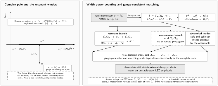
For $\delta=\Gamma_\star/M_\star\ll1$, residual momenta have size $M_\star\delta\sim\Gamma_\star$ while the resonant off-shellness has size $M_\star^2\delta\sim M_\star\Gamma_\star$. The pole $s_\star=M_\star^2-iM_\star\Gamma_\star$ supplies gauge-invariant matching input. The displayed $|z|\leq5$ interval is the companion benchmark’s accepted window, not a universal boundary; the general resonance condition is $z=O(1)$. Resonant, nonresonant, and observable-dependent soft or collinear terms must be combined at one declared order and attached to stable external states. The diagram is schematic and not to scale.

The resonant field makes width counting homogeneous

Remove the hard phase from the positive-frequency part of the scalar field, $\phi_v(x)=e^{iM_\star v\cdot x}P_+\phi(x)$. More generally, matching may use a renormalized mass $\widehat M$ different from the pole mass. Define the short-distance residual-mass coefficient

$$\Delta\equiv\frac{s_\star-\widehat M^2}{\widehat M} =\Delta^{(1)}+\Delta^{(2)}+\cdots.$$

In the pole scheme $\widehat M=M_\star$, one may parameterize $s_\star=M_\star^2-iM_\star\Gamma_\star$, so $\Delta=-i\Gamma_\star$ and $\Delta^{(1)}\sim M_\star\delta$. The leading resonant Lagrangian is

$$\mathcal L_{\mathrm{res}}^{(0)} =2M_\star\, \phi_v^\dagger \left(iv\!\cdot D_s-\frac{\Delta^{(1)}}{2}\right) \phi_v,$$

and its propagator is

$$\frac{i} {2M_\star\left(v\!\cdot k-\Delta^{(1)}/2\right)}.$$

With $\Delta^{(1)}=-i\Gamma_\star$, the pole is in the lower half-plane and the denominator contains $v\!\cdot k+i\Gamma_\star/2$. Both $v\!\cdot k$ and $\Delta^{(1)}$ are leading because they are the same size. This is the EFT origin of the fixed-width propagator; it is not an extra phenomenological insertion.

The first suppressed bilinear terms are

$$\begin{aligned} \mathcal L_{\mathrm{res}}^{(1)} =2M_\star\phi_v^\dagger \left[ \frac{(iD_{s\perp})^2}{2M_\star} +\frac{\left(\Delta^{(1)}\right)^2}{8M_\star} -\frac{\Delta^{(2)}}{2} \right]\phi_v, \end{aligned}$$

where $D_{s\perp}^\mu=D_s^\mu-v^\mu v\!\cdot D_s$. Each bracketed term is suppressed by one power of $\delta$ or the weak coupling relative to the leading inverse propagator. Beneke, Chapovsky, Signer, and Zanderighi derive this heavy-scalar effective Lagrangian, the production sources, and their matching in Beneke et al. 2004, §§ 2.1–2.3 and 3.1, preprint pp. 3–20, Open PDF.

The interaction Lagrangian has two topologies,

$$\mathcal L_{\mathrm{int}} =C_{\mathrm p}\,\mathcal O_{\mathrm p}\phi_v +C_{\mathrm d}\,\phi_v^\dagger\mathcal O_{\mathrm d} +\sum_a\frac{C_{\mathrm{nr},a}}{M_\star^{d_a-4}} \mathcal O_{\mathrm{nr},a} +\text{h.c.}+\cdots.$$

Production and decay operators contain a resonant field and stable energetic fields. Nonresonant operators contain only stable fields and represent the hard expansion of background topologies. The observable determines whether soft and collinear fields must also remain dynamical.

The homogeneous counting follows directly. In momentum space the resonant propagator scales as $\delta^{-1}$ after hard dimensions are removed, while $d^4k\sim\delta^4$. Requiring the quadratic action to be order one gives

$$\phi_v\sim\delta^{3/2}.$$

If the width-generating coupling obeys $\alpha\sim\delta$, two production or decay vertices and one resonant propagator give a normalized leading amplitude of order $\alpha/\delta\sim1$. A local nonresonant term has no $1/\delta$ enhancement and is therefore relatively of order $\delta$ in the scalar example. Hard corrections to $\Delta$ and $C_{\mathrm p,d}$, subleading bilinears, nonresonant operators, and soft loops can consequently enter at the same next-to-leading order. The long review gives the field scaling and this complete order assignment in Beneke 2015, §§ 1.1 and 2.1–2.4, article pp. 2–7, Open PDF.

First application: a scalar amplitude through first order

Use the dimensionful scalar benchmark

$$\mathcal A_{\mathrm{ref}}(s) =\frac{R}{s-s_p} +N +K\frac{s-M^2}{M^4},$$

with

$$s_p=\left(M-\frac{i\Gamma}{2}\right)^2, \qquad M=100, \qquad R=1, \qquad N=\frac{0.05}{M^2}, \qquad K=0.2.$$

This is a controlled algebraic fixture, not a physical line-shape model. It isolates the resonant pole, a local nonresonant term, and the first analytic energy-dependent remainder. At fixed scaled detuning

$$z=\frac{s-M^2}{M\Gamma}, \qquad \delta=\frac{\Gamma}{M},$$

the denominator is

$$s-s_p=M^2\delta\left(z+i+\frac{\delta}{4}\right).$$

Multiplying the amplitude by its leading resonant scale gives

$$M^2\delta\,\mathcal A_{\mathrm{ref}} =\frac{1}{z+i+\delta/4} +0.05\delta +0.2z\delta^2.$$

A strict width expansion through first relative order is therefore

$$\boxed{ M^2\delta\,\mathcal A_{\mathrm{ref}} =\frac{1}{z+i} +\delta\left[ 0.05-\frac{1}{4(z+i)^2} \right] +O(\delta^2) }.$$

The first term is the resonant leading amplitude. The term $-1/[4(z+i)^2]$ is the relative-$\delta$ correction obtained when the exact convention $s_p=(M-i\Gamma/2)^2$ is itself expanded; it is already present if the exact complex pole is retained in the leading denominator. The $0.05$ term is the local nonresonant contribution and is genuinely NLO relative to the enhanced pole. The analytic slope term proportional to $K$ begins at relative order $\delta^2$.

The registered benchmark adopts the pole-resummed convention

$$\mathcal A_{\mathrm{LO}}=\frac{1}{s-s_p}, \qquad \mathcal A_{\mathrm{NLO}}=\frac{1}{s-s_p}+\frac{0.05}{M^2},$$

and uses the $K$ term as an explicit NNLO remainder. At $z=1$, define

$$r(\delta) =\frac{|\mathcal A_{\mathrm{ref}}-\mathcal A_{\mathrm{NLO}}|} {|\mathcal A_{\mathrm{ref}}|}, \qquad p_i=\frac{\ln[r(2\delta_i)/r(\delta_i)]}{\ln2}.$$

Exact complex arithmetic gives

$\delta$	$r(\delta)$	Successive slope $p$
$0.005$	$7.0736823\times10^{-6}$	—
$0.010$	$2.8304889\times10^{-5}$	$2.00052$
$0.020$	$1.1329724\times10^{-4}$	$2.00099$
$0.040$	$4.5375226\times10^{-4}$	$2.00179$

The near-two slopes are not merely numerical evidence. At fixed $z$, the omitted term is $O(\delta/M^2)$ while the resonant amplitude is $O(1/(M^2\delta))$, so their ratio is $O(\delta^2)$. A numerical check should reproduce this scaling and explore its failure cases; the equations and table above also make the result checkable by hand.

Gauge independence belongs to the complete matched order

At NLO the amplitude is schematically

$$\mathcal A_{\mathrm{NLO}} =\mathcal A_{\mathrm{res}}^{(0)} +\mathcal A_{\Delta,C}^{(1)} +\mathcal A_{\mathrm{soft}}^{(1)} +\mathcal A_{\mathrm{nr}}^{(1)}.$$

The second term contains hard corrections to the pole coefficient, production and decay coefficients, and subleading resonant propagation. The third contains low-energy loops generated by the EFT. The fourth contains local nonresonant matching. Their separation is useful for power counting and single-scale calculations, but only the sum is a prediction.

In the scalar gauge-Yukawa example, expanding a hard self-energy beyond its pole term can cancel an adjacent resonant propagator. The resulting coefficient is gauge dependent until it is combined with hard vertex matching; at the next order, terms cancel both adjacent propagators and contribute to nonresonant matching. This is why a diagram cannot be classified once and for all as “resonant” or “background.” The EFT assigns each momentum region to a coefficient or matrix element and makes the required cancellation occur among operators of the same order. See Beneke 2015, § 2.3, article pp. 6–7, Open PDF.

A deliberately algebraic gauge-bookkeeping fixture makes the acceptance condition transparent:

$$\mathcal A_{\mathrm{res}}(\xi) =\mathcal A_0+\xi\delta\mathcal A_1, \qquad \mathcal A_{\mathrm{nr}}(\xi) =N_0-\xi\delta\mathcal A_1.$$

For any gauge parameter $\xi$,

$$\mathcal A_{\mathrm{res}}(\xi) +\mathcal A_{\mathrm{nr}}(\xi) =\mathcal A_0+N_0.$$

This identity is a unit test for cancellation, not a physical model of gauge dependence. A result that varies when $\xi=0,1,3$ is incomplete by construction.

The same counting specifies what is resummed. Since $\alpha M^2/(s-M^2)\sim\alpha/\delta\sim1$, the leading pole coefficient $\Delta^{(1)}$ belongs in the unperturbed resonant propagator. Higher pole terms, production and decay corrections, nonresonant operators, and soft loops are inserted at their assigned order. Resumming an arbitrary off-shell self-energy while omitting equally large vertex or nonresonant terms does not define an NLO approximation and can leave spurious gauge dependence. Only the two-point term responsible for the lifetime is forced into the leading Lagrangian; higher-point functions are not selectively resummed.

Validity window and matching limits

The single-resonance width expansion is controlled only when all of the following statements hold:

• $\delta=\Gamma_\star/M_\star\ll1$ and the width is generated in a perturbative sector whose coupling can be counted with $\delta$;
• the selected kinematics obey $z=(s-M_\star^2)/(M_\star\Gamma_\star)=O(1)$;
• the observable is defined using stable external states and is sufficiently specified to identify every soft, collinear, or measurement mode; and
• resonant, nonresonant, matching, and low-energy contributions are retained through one common target order.

The benchmark accepts $|z|\leq5$ to provide a deterministic test range. The number five is not a theorem. For $|z|\gg1$, the resonant propagator loses its $1/\delta$ enhancement and ordinary fixed-order perturbation theory is the appropriate expansion. A uniform result may be assembled schematically as

$$\mathcal A_{\mathrm{uniform}} =\mathcal A_{\mathrm{EFT}} +\mathcal A_{\mathrm{full}}^{[n]} -\left.\mathcal A_{\mathrm{EFT}}\right|_{\text{expanded to }[n]},$$

provided the full and EFT terms use compatible inputs, regulators, and subtraction conventions. The last term removes the overlap; an interpolation without this subtraction double counts the common fixed-order expansion.

Additional small scales require a larger theory. Near pair-production threshold, potential energy $Mv^2$ can be comparable to $\Gamma$ and Coulomb exchange may need resummation. A restrictive invariant-mass cut, jet veto, or endpoint measurement can resolve another scale of order $\Gamma$ and alter the mode content. A broad resonance with $\Gamma/M=O(1)$ has no width hierarchy, while an intrinsically nonperturbative resonance cannot obtain its matching coefficients from a weak-coupling pole expansion. These are stop conditions, not estimates of a larger truncation error.

Finally, never cut the resonant EFT propagator as though $\phi_v$ were an external state. The physical endpoint is a stable-decay-product observable of the type defined on Unstable-Particle Observables and Controlled Resonance Approximations. The method synthesis and scope on this page were checked through 3 August 2026; process-specific applications and live line-shape inputs are intentionally outside it.

Common pitfalls

Confusing $\Gamma$ with $M\Gamma$. Residual four-momentum is of order $\Gamma$, whereas virtuality is of order $M\Gamma$. Interchanging them breaks dimensions and the propagator counting.

Treating every nonresonant term as negligible. A local background lacks the resonant $1/\delta$ enhancement, but that makes it relatively NLO—not absent—in the scalar benchmark. Cuts or selection rules can change its order.

Calling a resummed propagator gauge invariant by itself. The complex pole is valid matching input. A selected off-shell self-energy and the diagrams built from it need not be gauge independent; the matched operator sum at a declared order must be.

Promoting the benchmark window to a law. $|z|\leq5$ is an executable test convention. The physical overlap with fixed order and any additional threshold or measurement scales determine the useful window in an application.

Exercises

1. Why does the resonant propagator scale as $1/(M^2\delta)$?

   Solution

   Near resonance, both $p^2-M^2$ and $M\Gamma$ are of order $M^2\delta$. The inverse denominator is therefore enhanced by $1/\delta$ relative to an ordinary hard propagator of order $1/M^2$.

2. Why are nonresonant operators required even inside the resonance window?

   Solution

   The same stable final state can be produced without the pole. Those hard contributions are not contained in production times resonant propagation times decay, and controlled matching requires their interference at the order assigned by the width counting.

References

• Beneke, Martin. 2015. “Unstable-Particle Effective Field Theory.” Nuclear and Particle Physics Proceedings 261–262: 218–231. DOI. Open PDF.

• Beneke, Martin, Alexander P. Chapovsky, Adrian Signer, and Giulia Zanderighi. 2004. “Effective Theory Calculation of Resonant High-Energy Scattering.” Nuclear Physics B 686 (1–2): 205–247. DOI. Open PDF.

• Stuart, Robin G. 1991. “Gauge Invariance, Analyticity and Physical Observables at the $Z^0$ Resonance.” Physics Letters B 262 (1): 113–119. DOI.