Multipole Expansion and Homogeneous Mode Power Counting

Separating momentum space into modes is not yet an effective theory. A mixed interaction generally contains components that vary on parametrically different coordinate scales. The slowly varying field must be expanded about the coordinates resolved by the fast field, and every common limit of two mode integrals must be subtracted. These two operations make the action homogeneous and make the momentum-space decomposition count each configuration once.

This page develops both operations at a fixed order in the small parameter $\lambda$. A two-mode scalar theory makes the counting transparent; gauge-covariant building blocks then show what changes in a gauge theory. The off-shell Sudakov triangle provides a summed-integrand check against expansion by regions.

Required background. Modes, Virtualities, and EFT Scale Separation supplies the mode scalings and Sudakov fixture. Power Counting and Predictive Order supplies the action-level counting rule used below.

Helpful background. Expansion by Regions develops the corresponding asymptotic expansion of individual integrals.

Projected coordinates and homogeneous fields

Choose null vectors $n^2=\bar n^2=0$ and $n\!\cdot\bar n=2$, and order light-cone components as

$$p\longleftrightarrow (n\!\cdot p,\bar n\!\cdot p,p_\perp).$$

An $n$-collinear momentum and an ultrasoft momentum scale as

$$p_c\sim Q(\lambda^2,1,\lambda), \qquad p_{us}\sim Q(\lambda^2,\lambda^2,\lambda^2).$$

The coordinates resolved by the collinear field therefore obey

$$(n\!\cdot x,\bar n\!\cdot x,x_\perp) \sim Q^{-1}(1,\lambda^{-2},\lambda^{-1}).$$

Define the two light-cone projections

$$x_-^\mu=\frac{\bar n\!\cdot x}{2}n^\mu, \qquad x_+^\mu=\frac{n\!\cdot x}{2}\bar n^\mu.$$

Across an $n$-collinear interaction, the ultrasoft phase has the hierarchy

$$p_{us}\!\cdot x_-=O(1), \qquad p_{us\perp}\!\cdot x_\perp=O(\lambda), \qquad p_{us}\!\cdot x_+=O(\lambda^2).$$

Thus an ultrasoft scalar field in that interaction has the multipole expansion

$$\begin{aligned} \phi_{us}(x) ={}&\phi_{us}(x_-) +x_\perp\!\cdot\partial_\perp\phi_{us}(x_-) +\frac{n\!\cdot x}{2}\,\bar n\!\cdot\partial\,\phi_{us}(x_-) \\ &+\frac12x_\perp^\mu x_\perp^\nu \partial_{\perp\mu}\partial_{\perp\nu}\phi_{us}(x_-) +O(\lambda^3). \end{aligned}$$

The displayed corrections are respectively suppressed by $\lambda$, $\lambda^2$, and $\lambda^2$ relative to the first term. The expansion does not restrict the coordinate integral to a small region. It replaces one nonhomogeneous interaction by a series of operators, each with a definite power. A truncation is translation invariant up to terms beyond its declared accuracy.

Object	Component scaling	Coordinate consequence	Role in the expansion
$n$-collinear field	$Q(\lambda^2,1,\lambda)$	Resolves $n\!\cdot x$, $\bar n\!\cdot x$, and $x_\perp$ at three different scales	Kept at the full interaction coordinate $x$
Ultrasoft field	$Q(\lambda^2,\lambda^2,\lambda^2)$	Varies at leading order only along $x_-$ inside an $n$-collinear interaction	Evaluated at $x_-$ and expanded in transverse and $x_+$ displacements
$\bar n$-collinear field	$Q(1,\lambda^2,\lambda)$	Interchanges the two light-cone coordinate roles	Couples to an ultrasoft field evaluated at $x_+$

First application: a two-mode scalar interaction

Consider massless scalar $\phi^3$ theory in $d=6$,

$$\mathcal L =\frac12\partial_\mu\phi\,\partial^\mu\phi -\frac{g}{3!}\phi^3.$$

Six dimensions make $g$ dimensionless, so no coupling convention obscures the mode counting. Split the field into $n$-collinear, $\bar n$-collinear, and ultrasoft components. Momentum conservation permits the same-direction mixed interactions $\phi_c^2\phi_{us}$ and $\phi_{\bar c}^2\phi_{us}$, while interactions whose large light-cone momenta cannot sum to the declared external scaling are absent.

The cited scalar construction calls the all-components-$Q\lambda^2$ field “soft.” This chapter uses the component-explicit name ultrasoft for that scaling; no physics changes with the label.

The kinetic actions fix

$$\phi_c\sim Q^2\lambda^2, \qquad \phi_{us}\sim Q^2\lambda^4, \qquad d^6x_c\sim Q^{-6}\lambda^{-6}.$$

The $n$-collinear mixed action becomes

$$\begin{aligned} S_{c,us} =-\frac g2\int d^6x\,\phi_c^2(x) \bigg[ &\phi_{us}(x_-) +x_\perp\!\cdot\partial_\perp\phi_{us}(x_-) \\ &+\frac{n\!\cdot x}{2}\bar n\!\cdot\partial\,\phi_{us}(x_-) +\frac12x_\perp^\mu x_\perp^\nu \partial_{\perp\mu}\partial_{\perp\nu}\phi_{us}(x_-) +\cdots \bigg]. \end{aligned}$$

Every line is homogeneous:

Scalar operator in $S_{c,us}$	Relative factor inside brackets	Action scaling
$\phi_c^2\phi_{us}(x_-)$	$1$	$g\lambda^2$
$\phi_c^2x_\perp\!\cdot\partial_\perp\phi_{us}(x_-)$	$\lambda$	$g\lambda^3$
$\phi_c^2(n\!\cdot x)\bar n\!\cdot\partial\,\phi_{us}(x_-)/2$	$\lambda^2$	$g\lambda^4$
$\phi_c^2x_\perp^\mu x_\perp^\nu\partial_{\perp\mu}\partial_{\perp\nu}\phi_{us}(x_-)/2$	$\lambda^2$	$g\lambda^4$

For example, the leading term scales as

$$g\,(Q^{-6}\lambda^{-6}) (Q^2\lambda^2)^2(Q^2\lambda^4) =g\lambda^2.$$

The $\bar n$-collinear interaction follows by $n\leftrightarrow\bar n$ and $x_-\leftrightarrow x_+$. This calculation verifies two separate statements: the first mixed scalar interaction is power suppressed relative to the sector kinetic actions, and its derivative corrections advance in definite powers of $\lambda$. Becher, Broggio, and Ferroglia derive this scalar construction, including the projected coordinate and leading Lagrangian, in Becher, Broggio, and Ferroglia 2015, § 3.1, preprint pp. 18–20, Open PDF.

Gauge-covariant multipoles

An ordinary Taylor series of a charged field is not gauge covariant because fields at $x$ and $x_-$ transform at different points. Parallel transport first. With $D_\mu=\partial_\mu-igA_\mu$, define a straight Wilson line from $x$ to $x_-$,

$$[x_-,x] =P\exp\!\left(ig\int_x^{x_-}\!dz^\mu A_\mu(z)\right).$$

The combination $[x_-,x]\Phi(x)$ transforms at $x_-$. Its covariant expansion is

$$[x_-,x]\Phi(x) =\Phi(x_-) +\Delta x^\mu D_\mu\Phi(x_-) +\frac12\Delta x^\mu\Delta x^\nu D_{(\mu}D_{\nu)}\Phi(x_-) +\cdots, \qquad \Delta x=x-x_-.$$

Equivalently, one can build the EFT from Wilson-line-dressed fields, covariant derivatives, and field strengths before sorting by $\lambda$. In leading-power soft-collinear QCD, the component comparison gives

$$i n\!\cdot D =i n\!\cdot\partial +g\,n\!\cdot A_c(x) +g\,n\!\cdot A_{us}(x_-),$$

while other ultrasoft gauge-field components are suppressed in the $n$-collinear Lagrangian. Gauge transformations must be multipole expanded with the fields, and all operators at one power must be retained together. Becher, Broggio, and Ferroglia give the leading soft-collinear replacement, expanded gauge transformations, Wilson-line transformation law, and invariant building blocks in Becher, Broggio, and Ferroglia 2015, §§ 4.3–4.5 and 4.8, preprint pp. 34–45, Open PDF.

This rule prevents a common false shortcut: replacing $A_{us}(x)$ by $A_{us}(x_-)$ is not, by itself, a gauge-invariant approximation. The transformation law, Wilson lines, and subleading insertions must be expanded to the same order.

Overlap and zero-bin subtraction

Multipole expansion makes each mode integral homogeneous, but homogeneous domains still extend over all momentum space after regularization. Their common limits can therefore be counted twice. In label language, the zero label of a collinear field is excluded because that momentum belongs to the ultrasoft field. When the sum over nonzero labels is replaced by an unrestricted integral, the missing restriction reappears as a subtraction.

Let $T_cF$ be the collinear expansion of a full integrand $F$, and let $T_{us}$ expand that result in its ultrasoft limit. The subtracted collinear integrand is

$$F_c^{\mathrm{sub}} =T_cF-T_{us}T_cF.$$

For several intersecting limits, use inclusion–exclusion:

$$F^{\mathrm{sub}} =F-\sum_iF_i^{(0)} +\sum_{i<j}F_{ij}^{(0)} -\sum_{i<j<k}F_{ijk}^{(0)}+\cdots.$$

The scaling limit is taken and expanded at the level of the complete graph integrand after momentum-conserving constraints are imposed. Subtracting one expression per loop momentum can miss overlaps associated with individual propagator labels. Manohar and Stewart formulate this construction and its nested subtractions in Manohar and Stewart 2007, § IV, preprint pp. 17–20, Open PDF.

An overlap subtraction is not hard matching. It reallocates a long-distance configuration among retained modes; matching removes short-distance fluctuations. Finite pieces can move between sectors under an overlap scheme change, but the matched physical sum cannot.

Sudakov check against expansion by regions

Return to the off-shell Sudakov triangle with

$$P^2\sim L^2\sim\lambda^2Q^2.$$

Write $\widetilde I_c$ for the naive $n$-collinear integral and

$$I_{c,0} =i\pi^{-d/2}\mu^{2\epsilon} \int d^dk\,T_{us}T_cF(k)$$

for its ultrasoft zero-bin. At leading power, systematic expansion makes this overlap homogeneous with no remaining scale, so $I_{c,0}=0$ in dimensional regularization. The $\bar n$-collinear overlap vanishes for the same reason. Therefore

$$I_{\mathrm{EFT}}^{(0)} =(\widetilde I_c-I_{c,0}) +(\widetilde I_{\bar c}-I_{\bar c,0}) +I_{us} =I_c+I_{\bar c}+I_{us}.$$

Adding the hard matching contribution gives exactly the leading expansion-by-regions result,

$$I_h+I_{\mathrm{EFT}}^{(0)} =\frac1{Q^2} \left[ \ln\frac{Q^2}{L^2}\ln\frac{Q^2}{P^2} +\frac{\pi^2}{3} \right] +O(\lambda).$$

The zero value is a checked property of this integrand, power, and regulator—not permission to omit the subtraction rule. A measurement boundary, mass, rapidity regulator, or incompletely expanded denominator can supply a scale and make the zero-bin nonzero. Becher, Broggio, and Ferroglia show the scaleless overlaps and summed region result in Becher, Broggio, and Ferroglia 2015, § 2.2, preprint pp. 9–15, Open PDF.

The construction map

In the figure, the left panel supplies the component scalings used above. In the right panel, inspect the third step: multipole expansion and overlap subtraction are both required before sector matching or evolution. The scalar calculation realizes its multipole half, while the Sudakov zero-bin realizes its overlap half.

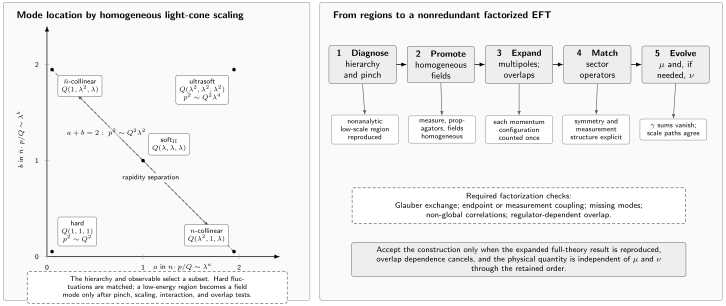
Mode locations are shown in the exponents $a$ and $b$ of $(n\!\cdot p/Q,\bar n\!\cdot p/Q)\sim(\lambda^a,\lambda^b)$, with the transverse exponent written in each label. The line $a+b=2$ contains $n$-collinear, $\bar n$-collinear, and soft-II scalings of virtuality $Q^2\lambda^2$; their separation along the line is a rapidity separation. Ultrasoft momentum has virtuality $Q^2\lambda^4$, while hard fluctuations are matched at $Q^2$. The points are alternatives selected by a hierarchy and observable, not a universal simultaneous field list. A consistent construction requires homogeneous fields, multipole and overlap expansion, sector matching, and $\mu$ and, when needed, $\nu$ evolution, with explicit factorization checks. The diagram is schematic and not to scale.

A fixed-order construction test

Before accepting a mode Lagrangian through $O(\lambda^N)$, verify all of the following:

• every field, derivative, measure, coupling, source, and measurement has a declared scaling;
• every slow field in a mixed interaction is projected and expanded through the order that can contribute to $\lambda^N$;
• gauge transformations and Wilson-line building blocks are expanded to the same order;
• momentum conservation allows each retained operator, and the action—not merely its Lagrangian density—is homogeneous;
• all pairwise and nested zero-bins are generated from the complete integrand;
• regulator dependence and any overlap-scheme dependence cancel in the matched sum; and
• at least one amplitude or integral reproduces the corresponding expansion-by-regions result.

Common pitfalls

Expanding the fast field instead of the slow field. The relevant comparison is between derivative scaling and the coordinates resolved by the interaction. For an $n$-collinear interaction, the ultrasoft field is slow in $x_\perp$ and $x_+$ but not along $x_-$.

Dropping every scaleless zero-bin before constructing it. A scaleless integral can encode canceling ultraviolet and infrared poles, and a measurement can make the same limit non-scaleless. Form the subtraction first and then evaluate it in the declared regulator.

Using an ordinary Taylor series for gauge fields. Terms at different spacetime points do not transform together. Parallel transport to a common point or use gauge-covariant EFT building blocks before truncating.

Counting the density but not the action. Different modes have different coordinate measures. Operator order follows only after the field scalings and the appropriate integration measure are included.

Exercises

1. Why is the transverse ultrasoft correction suppressed by one power of $\lambda$ in the scalar example?

   Solution

   The collinear coordinate scales as $x_\perp\sim1/(Q\lambda)$ while the ultrasoft derivative scales as $\partial_{us,\perp}\sim Q\lambda^2$. Hence $x_\perp\!\cdot\partial_{us,\perp}\sim\lambda$.

2. Which momentum components are conserved at the leading mixed vertex?

   Solution

   The large collinear label momenta are conserved separately because ultrasoft momentum cannot change them. The residual collinear components and ultrasoft momentum obey the remaining momentum-conservation relation.

References

• Becher, Thomas, Alessandro Broggio, and Andrea Ferroglia. 2015. Introduction to Soft-Collinear Effective Theory. Lecture Notes in Physics 896. Cham: Springer. DOI. Open PDF.

• Manohar, Aneesh V., and Iain W. Stewart. 2007. “The Zero-Bin and Mode Factorization in Quantum Field Theory.” Physical Review D 76 (7): 074002. DOI. Open PDF.