A Map of Effective-Theory Architectures

An effective theory is chosen by the low-energy problem, not by resemblance to a familiar Lagrangian. The decisive data are the degrees of freedom that can propagate or remain slow, the hierarchy that makes an expansion small, the realization of symmetry and state information, and the observable whose accuracy must be controlled. This page turns those data into a selection algorithm and a comparison map spanning relativistic contact theories, chiral and nuclear EFTs, heavy and nonrelativistic particles, SCET, electroweak EFTs, gravity, hydrodynamics, open systems, and many-body patch theories.

Required background. Effective Field Theory as a Controlled Expansion supplies the operator, matching, and remainder logic used in every architecture card.

Helpful background. EFT Truncation Errors and Breakdown Diagnostics explains how a nominal expansion becomes an error statement. Integrating Out Heavy Fields develops the local heavy-mass limit. From Operator Lists to Independent Bases separates a symmetry-allowed list from a nonredundant basis.

An architecture is a tuple, not an acronym

For a proposed EFT, record the architecture card

\mathfrak A =\bigl(\mathcal D,\mathcal H,\mathcal S,\mathcal P, \mathcal M,\mathcal O,\mathcal U,\mathcal R\bigr).

Its entries are:

$\mathcal D$ : retained fields, modes, collective variables, or density-matrix data;
$\mathcal H$ : dimensionless scale ratios and the kinematic or state hierarchy;
$\mathcal S$ : symmetry realization, locality, gauge redundancy, and—when relevant—the time contour or reduced state;
$\mathcal P$ : the counting assigned to derivatives, masses, fields, loops, insertions, and iterations;
$\mathcal M$ : matching conditions or empirical inputs that determine coefficients and matrix elements;
$\mathcal O$ : observables or correlation functions for which the construction closes;
$\mathcal U$ : truncation uncertainty, diagnostics, and a breakdown condition; and
$\mathcal R$ : the subject page that develops coefficients, dynamics, data, and validation.

Two theories may share an operator while having different cards. A four-fermion interaction can be a weak-scale contact operator, a promoted interaction in a shallow two-body channel, or a marginal coupling between Fermi-surface patches. Its canonical mass dimension does not determine its order in those distinct scaling limits, so the written monomial does not select the architecture. The general principle—that low-energy fields and power counting are fixed by scale separation and matching rather than by a finite list of renormalizable interactions—is developed in Manohar 2018, §§ 2.3–2.8 and 3.1–3.5, preprint pp. 9–31, Open PDF.

The figure shows the selection logic. Start at the observable and state, identify the structure that organizes the low-energy limit, and then complete the same card regardless of the branch. Inspect especially the dashed region: its branches are alternatives that may also be nested, not successive mandatory stages.

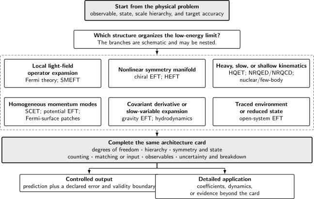
The organizing feature of a low-energy problem selects one or more EFT architecture branches, but every branch must complete the same card before producing a controlled prediction and linking onward to detailed applications. — An EFT name is not a construction. Starting from the observable, state, scale hierarchy, and target accuracy, identify the dominant low-energy organizing structure, then declare degrees of freedom, symmetry and state, counting, matching or input, observables, uncertainty, and breakdown. Branches may be nested; the diagram is schematic and not to scale.

A selection algorithm

Apply the following sequence before writing an EFT Lagrangian.

Fix the output. State the amplitude, rate, spectrum, bound-state level, response function, transport coefficient, or reduced-state observable, together with its kinematic region and target accuracy. An EFT valid for an inclusive rate need not close for an endpoint distribution, and a theory for amplitudes need not determine an open-system density matrix.
Retain every low-energy carrier. Keep fields that can go on shell, modes selected by pinch surfaces, Goldstone coordinates required by spontaneous symmetry breaking, conserved slow variables, shallow bound-state channels, and system variables whose environment has been traced out. Integrate out only fluctuations separated by the declared hierarchy.
Name the small parameters. Examples are $E/M_W$ , $Q/\Lambda_\chi$ , $\Lambda_{\mathrm{QCD}}/m_Q$ , a nonrelativistic velocity $v$ , a collinear parameter $\lambda$ , curvature in cutoff units, $\omega\tau_{\mathrm{micro}}$ , or a system–environment time-scale ratio. If no dimensionless ratio is small, a formal operator expansion is not yet controlled.
Specify symmetry, state, and locality. Decide whether a symmetry is linearly or nonlinearly realized, whether reference vectors or patches introduce redundancies, whether the action is local after the relevant expansion, and whether a closed-time-path doubling is required. These choices can distinguish architectures even when their particles are identical.
Close the counting under quantum corrections and required iterations. Assign orders to every building block and verify that loops and any nonperturbative resummation generate counterterms at predicted orders. A shallow pole can promote a contact interaction; equal-virtuality modes can require rapidity rather than ordinary virtuality counting.
Declare how short-distance information enters. Matching may compare amplitudes, Green functions, background-field functionals, potentials, influence kernels, or correlation functions. Some low-energy constants instead come from data or lattice calculations. State the scale, scheme, states, and retained order.
Test an observable. Construct at least one quantity in which unphysical basis, regulator, gauge, frame, label, or matching-scale dependence cancels to the stated order.
Attach an uncertainty and a validity boundary. Separate omitted EFT orders from perturbative matching, input, numerical, state-preparation, and model errors. Stop when an omitted mode becomes light, a hierarchy collapses, an iteration is no longer renormalized, memory becomes important, or the requested observable leaves the proven factorization domain.
Route the application. The architecture page explains why the EFT has its form. Continue to the exact subject page for numerical coefficients, fits, material-specific dynamics, and phenomenological validation.

This order is intentionally observable-first. Starting from “all operators allowed by symmetry” can miss a mode, an infrared enhancement, a state constraint, or an iteration that changes the counting.

Architecture comparison matrix

The matrix is a compact decision aid, not a substitute for constructing the card. “Breakdown” means the first assumption whose failure invalidates the stated expansion; it is not always the largest mass in the microscopic theory.

Framework	Degrees of freedom	Hierarchy or state	Symmetry and locality	Power counting	Matching or input	Representative outputs	Uncertainty and validity limit	Detailed application
Fermi contact EFT	Light quarks and leptons; photons and gluons when required	$E/M_W\ll1$ below weak thresholds	Local operators invariant under unbroken color and electromagnetism	Canonical dimension, couplings, and loops	Match the Standard Model or determine $G_F$ and flavor inputs	Weak decays and low-energy scattering	Higher powers of $E^2/M_W^2$ , perturbative matching, and inputs; stop near weak thresholds	The Fermi Limit of Weak Interactions
Chiral EFT	Goldstone bosons, with matter fields added only for the target process	$Q/\Lambda_\chi\ll1$ and explicit-breaking ratios	Nonlinear realization on $G/H$ ; local derivative expansion	Derivatives, light masses, and loops in chiral order	Low-energy constants from QCD, lattice calculations, or data	Soft-pion amplitudes and low-energy hadron observables	Next chiral order and input errors; stop when non-Goldstone modes or hard momenta are resolved	Chiral Lagrangians and Low-Energy QCD
Nuclear and few-body EFT	Nucleons, possibly pions or auxiliary shallow-channel fields	$Q/\Lambda_b\ll1$ plus unnaturally large scattering lengths or shallow poles	Galilean or Lorentz remnants, internal symmetries, and sometimes nonlinear chiral symmetry	Promoted contacts and nonperturbative iteration, then range or chiral corrections	Few-body data, lattice QCD, and QCD-constrained inputs	Scattering, bound states, and nuclear forces	Order-by-order cutoff independence and truncation; stop when omitted pion, excitation, or inelastic scale is resolved	Nuclear Forces and the Chiral Expansion
HQET	Velocity-labelled heavy field $h_v$ and light QCD fields	Residual momentum $k\sim\Lambda_{\mathrm{QCD}}\ll m_Q$	Gauge symmetry, heavy-quark spin–flavor symmetry at leading order, and reparameterization constraints	$\Lambda_{\mathrm{QCD}}/m_Q$ with perturbative coefficient running	Match QCD at $m_Q$ ; nonperturbative hadron matrix elements	Heavy-hadron symmetry relations and decay expansions	Higher $1/m_Q$ orders, matching, and matrix elements; stop without a heavy–residual hierarchy	Heavy-Quark Symmetry and HQET
NRQED, NRQCD, and potential EFT	Pauli heavy particles; for pairs, potential, soft, and ultrasoft modes as needed	$v\ll1$ with $m\gg mv\gg mv^2$ when weak coupling applies	Gauge and rotational symmetry with nonrelativistic field content	Velocity, $1/m$ , multipole, and loop counting	Match at $m$ , then at $mv$ when constructing a potential EFT	Spectra, threshold rates, decays, and radiative transitions	Missing velocity orders, matching, potentials, and nonperturbative inputs; stop when scale separation or a potential description fails	Bound-State QED and NRQED and Quarkonium and Nonrelativistic QCD
SCET	One collinear sector per resolved direction plus soft, ultrasoft, collinear-soft, or Glauber modes selected by the observable	Homogeneous momentum scalings in $\lambda$ ; sometimes equal virtuality but separated rapidity	Sector gauge symmetries, multipole locality, Wilson lines, and overlap subtraction	Homogeneous $\lambda$ scaling with virtuality and, when required, rapidity evolution	Hard and staged mode matching; measured sector matrix elements	Endpoint spectra, jet observables, and factorized amplitudes	Power corrections, overlap and scale consistency, endpoints, and Glauber tests; stop outside the proven measurement domain	Soft-Collinear Effective Theory: Architecture and Validity
SMEFT and HEFT	Standard Model fields; HEFT treats electroweak Goldstones nonlinearly and the scalar separately	$Q/\Lambda\ll1$ with $Q\in\{E,v,m,\ldots\}$	Linear Higgs-doublet realization in SMEFT; nonlinear electroweak realization in HEFT	Canonical dimension in SMEFT; chiral and loop order in HEFT	Match a UV theory or infer coefficients in a declared input scheme	Electroweak and Higgs amplitudes and pseudo-observables	EFT, loop, basis, input-scheme, and fit errors; stop at new thresholds or when the assumed scalar geometry fails	SMEFT and HEFT in Standard Model Observables
Gravity EFT	Metric fluctuations and all light matter fields	$E/\Lambda_g\ll1$ and curvature small in cutoff units	Diffeomorphism invariance and a local covariant derivative expansion	Derivatives, curvature insertions, and loops	Wilson coefficients from a UV theory or measurement; massless nonanalytic terms are low-energy predictions	Low-energy scattering and long-distance corrections	Higher derivatives, loops, and coefficient inputs; stop at strong curvature, new light states, or the cutoff	Applying EFT Power Counting to Gravity
Hydrodynamic EFT	Conserved slow densities or fluid maps, with doubled variables for fluctuations and dissipation	$\omega\tau_{\mathrm{micro}}\ll1$ and $k\ell_{\mathrm{micro}}\ll1$ near a specified state	Conservation laws, gauge and diffeomorphism covariance, closed-time-path constraints, and thermal KMS symmetry when applicable	Gradients, amplitudes, and fluctuations	Equation of state, susceptibilities, and transport data	Hydrodynamic modes, response functions, noise, and constitutive relations	Higher gradients, fluctuations, and transport inputs; stop when nonhydrodynamic modes or instabilities enter	Schwinger–Keldysh Effective Actions for Fluids
Open-system EFT	Reduced density matrix or doubled system fields after environmental variables are traced out	Separation of system and environment scales, with a declared initial state and memory regime	Trace preservation, Hermiticity, causality, and positivity constraints; locality in time needs an extra approximation	Coupling, derivatives, noise, and memory expansion	Trace out the environment or determine influence kernels from microscopic theory or data	Reduced correlators, dissipation, decoherence, and stochastic dynamics	Kernel truncation, initial correlations, positivity, and memory; stop when a Markovian or local approximation fails	System–Environment Splits and Influence Functionals
Many-body and patch EFT	Quasiparticles, Fermi-surface patches, order parameters, or emergent gauge and collective modes	Energy relative to $E_F$ , distance normal to the Fermi surface, or distance to a critical scale	Microscopic and emergent symmetries with patch or lattice kinematics	Patch scaling, derivatives, loops, and sometimes large- $N$ or epsilon expansions	Microscopic models, lattice calculations, or experimental response	Phases, instabilities, collective modes, and response functions	Patch, quasiparticle, and critical-expansion errors; stop when the retained low-energy manifold changes	Fermi-Surface Patch Theory and Low-Energy Scaling

Several entries require qualifications that the compact cells cannot carry. Chiral loops follow the same derivative hierarchy as symmetry-allowed counterterms, but shallow nuclear channels introduce infrared enhancement and nonperturbative iteration; Epelbaum, Hammer, and Meißner 2009, §§ I.D and II.A, pp. 1778–1780 and 1784–1787 explain why nuclear counting cannot be inferred from the pion theory alone. HQET retains the nearly on-shell heavy quark by writing $p_Q=m_Qv+k$ , while potential theories resolve the distinct $m$ , $mv$ , and $mv^2$ scales of a heavy pair; see Neubert 1996, § 3, printed pp. 18–21, Open PDF and Pineda 2012, §§ 1–3, pp. 735–749.

Likewise, SCET begins from homogeneous collinear and long-wavelength momentum regions rather than from a heavy-mass expansion Bauer et al. 2001, §§ I–II, pp. 1–8, Open PDF. SMEFT and HEFT differ in symmetry realization and therefore in counting, not merely in basis notation Brivio and Trott 2019, §§ 5–6, pp. 46–71 and Buchalla, Catà, and Krause 2014, §§ 3 and 5, pp. 556–564. In gravity, local higher-curvature coefficients coexist with nonanalytic long-distance effects of massless propagation Donoghue 1994, § 3, preprint pp. 5–9, Open PDF.

State information becomes constitutive in the last three rows. A fluctuating dissipative fluid uses doubled variables and, for thermal states, a local KMS condition Crossley, Glorioso, and Liu 2017, §§ I–II, pp. 1–13, Open PDF. Tracing environmental states gives a reduced density matrix, but a local Markovian or Lindblad equation needs assumptions beyond the partial trace Braaten, Hammer, and Lepage 2016, § II.B, pp. 3–4. A Fermi surface instead leaves a codimension-one manifold of low-energy modes, so scaling is toward the surface rather than uniformly toward zero momentum Polchinski 1992, pp. 12–16, Open PDF.

Rejecting near matches

A useful architecture map must say “no” as well as “yes.” The following pairs are superficially similar but fail different card entries.

HQET is not generic nonrelativistic EFT. HQET describes a single heavy quark exchanging residual momentum of order $\Lambda_{\mathrm{QCD}}$ with light degrees of freedom; its reference velocity is fixed at leading order. A near-threshold heavy particle–antiparticle pair has kinetic energy $mv^2$ , potential momentum $mv$ , annihilation operators, and possibly a Schrödinger potential. Using HQET for quarkonium loses the pair hierarchy; using NRQCD for an isolated heavy–light hadron hides the leading heavy-quark symmetry.

Pion chiral EFT is not automatically nuclear EFT. A perturbative derivative expansion around soft Goldstone interactions does not reproduce a large nucleon scattering length by finite-order insertions. Shallow poles demand promoted interactions and iteration. Conversely, a pionless contact theory ceases to be complete when the pion range is resolved.

SMEFT and HEFT are not two labels for the same basis. SMEFT assumes that the Higgs belongs to a linearly transforming doublet and expands local operators by canonical dimension. HEFT allows a nonlinear electroweak Goldstone manifold with an independent scalar function and uses chiral/loop counting. A nonlinear field redefinition can relate descriptions only within a patch where it is regular and where the assumed scalar geometry admits the linear organization; it cannot erase a genuine difference in the low-energy manifold.

Hydrodynamic EFT is not a synonym for open-system EFT. Hydrodynamics is selected by conserved quantities and the derivative expansion around a state. An open EFT is selected by a system–environment split and reduced dynamics. A fluid can require open-system machinery to encode dissipation and noise, but an open qubit has no hydrodynamic conserved-mode expansion, while an ideal closed fluid need not be introduced by tracing out a named environment.

SCET modes are not fields chosen only by small invariant mass. Two regions can have equal virtuality yet be separated in rapidity, and a Glauber or collinear-soft mode may be required by pinches or measurements. Integrating all low-virtuality radiation into one field can double count an overlap or omit a leading region even when every individual momentum is “soft.”

First application: classify Fermi theory

Consider a charged-current process at momentum transfer $|q^2|\sim E^2\ll M_W^2$ . The full-theory propagator contains

\frac{1}{M_W^2-q^2} =\frac{1}{M_W^2} \left(1+\frac{q^2}{M_W^2} +O\!\left(\frac{q^4}{M_W^4}\right)\right).

After integrating out the $W$ , a convenient low-energy convention is

\mathcal L_F =-\frac{4G_F}{\sqrt2}\,V_{ij} \bigl(\bar u_i\gamma^\mu P_Ld_j\bigr) \bigl(\bar\ell\gamma_\mu P_L\nu_\ell\bigr) +\text{h.c.}, \qquad \frac{G_F}{\sqrt2}=\frac{g^2}{8M_W^2}

at tree level, before process-dependent electroweak, QCD, and QED corrections. The card is now explicit:

Entry	Fermi-theory choice
Degrees of freedom $\mathcal D$	External light quarks and leptons, plus photons and gluons when their low-energy corrections are resolved; the $W$ is absent.
Hierarchy $\mathcal H$	$E/M_W\ll1$ , with any additional hadronic or lepton thresholds declared for the process.
Symmetry and locality $\mathcal S$	A local operator expansion invariant under the unbroken low-energy gauge symmetries; the weak interaction appears through left-handed currents and flavor data.
Counting $\mathcal P$	The leading current product has dimension six and coefficient $O(M_W^{-2})$ ; derivative corrections begin at relative order $E^2/M_W^2$ , while loops carry their own coupling expansion.
Matching or input $\mathcal M$	Match the full charged-current amplitude at a weak scale, evolve if scales are widely separated, and use a declared definition of $G_F$ , CKM factors, and hadronic matrix elements.
Observable $\mathcal O$	A specified low-energy decay or scattering amplitude, not the coefficient alone.
Uncertainty $\mathcal U$	Separate omitted $E^2/M_W^2$ terms, perturbative matching/running, CKM and other inputs, and hadronic matrix elements. Stop as $E$ approaches a weak threshold or an omitted particle becomes dynamical.
Route $\mathcal R$	The weak-interaction application and normalization belong to The Fermi Limit of Weak Interactions; generic matching and counting remain here in Volume 5.

This example selects the local light-field operator branch in the figure. It does not select HQET merely because a heavy $W$ appears in the microscopic theory: HQET retains a heavy external particle, whereas the Fermi construction removes the mediator. It also does not select SMEFT for the low-energy calculation itself: SMEFT keeps the full Standard Model field content and electroweak gauge symmetry above the weak scale, while the Fermi theory lives below electroweak thresholds. A multistage analysis may nevertheless match a UV model to SMEFT, then to a low-energy weak Hamiltonian, and finally to hadronic or nuclear EFT. The branches can therefore be nested without becoming interchangeable.

Validity checks and boundaries

Before accepting any architecture assignment, require five checks:

Spectrum check: every state or mode that can become on shell in the declared domain is retained or represented by a justified nonlocal structure.
Counting check: loops and mandatory iterations generate only operators included at the predicted order, with regulator dependence absorbed by available counterterms.
Symmetry check: the chosen linear, nonlinear, gauge, contour, or frame realization survives regularization and matching.
Observable check: auxiliary choices cancel in at least one computed quantity to the claimed order.
Boundary check: approaching the first omitted threshold or failure regime visibly degrades the expansion or triggers a planned rematching.

This page deliberately does not provide a catalog of models, current coefficient fits, or numerical low-energy constants. Those data change by process and are developed in the application linked from the last column. Nor does the map imply that every problem has a unique single branch: heavy-to-light decays can combine HQET and SCET, nuclear reactions can combine chiral and few-body counting, and fluctuating hydrodynamics combines slow-variable and closed-time-path structures. The requirement is that the composed card be internally consistent and that each approximation retain its own validity limit.

Common pitfalls

Choosing by particle names. “There is a heavy particle” does not distinguish decoupling, HQET, NRQCD, and a resonance EFT. Ask whether the particle is removed, remains nearly on shell with fixed velocity, participates in a nonrelativistic pair, or is unstable in the measured region.

Using canonical dimension as universal counting. Canonical dimension organizes a local relativistic contact expansion such as Fermi theory or SMEFT. Infrared enhancement, nonlinear symmetry, velocity scaling, patch scaling, or gradients can promote operators and require a different order assignment.

Treating matching as the prediction. A Wilson coefficient is only one card entry. The result also needs low-energy matrix elements, evolution, an observable definition, and an uncertainty with a breakdown condition.

Forcing locality after tracing or factorizing. Integrating out a gapped heavy field admits a local derivative expansion below threshold. Tracing an environment or separating momentum sectors can instead leave memory kernels, Wilson lines, potentials, or measurement-dependent nonlocality; locality must be derived in the relevant variables.

References

Bauer, Christian W., Sean Fleming, Dan Pirjol, and Iain W. Stewart. 2001. “An Effective Field Theory for Collinear and Soft Gluons: Heavy to Light Decays.” Physical Review D 63 (11): 114020. DOI. Open PDF.
Braaten, Eric, H.-W. Hammer, and G. Peter Lepage. 2016. “Open Effective Field Theories from Deeply Inelastic Reactions.” Physical Review D 94 (5): 056006. DOI. Open PDF.
Brivio, Ilaria, and Michael Trott. 2019. “The Standard Model as an Effective Field Theory.” Physics Reports 793: 1–98. DOI. Open PDF.
Buchalla, Gerhard, Oscar Catà, and Claudius Krause. 2014. “Complete Electroweak Chiral Lagrangian with a Light Higgs at NLO.” Nuclear Physics B 880: 552–573. DOI. Open PDF.
Crossley, Michael, Paolo Glorioso, and Hong Liu. 2017. “Effective Field Theory of Dissipative Fluids.” Journal of High Energy Physics 2017 (9): 095. DOI. Open PDF.
Donoghue, John F. 1994. “General Relativity as an Effective Field Theory: The Leading Quantum Corrections.” Physical Review D 50 (6): 3874–3888. DOI. Open PDF.
Epelbaum, Evgeny, Hans-Werner Hammer, and Ulf-G. Meißner. 2009. “Modern Theory of Nuclear Forces.” Reviews of Modern Physics 81 (4): 1773–1825. DOI. Open PDF.
Manohar, Aneesh V. 2018. “Introduction to Effective Field Theories.” Les Houches lecture notes. arXiv:1804.05863. Open PDF.
Neubert, Matthias. 1996. “Heavy-Quark Effective Theory.” CERN-TH/96-281, lectures presented at the 34th International School of Subnuclear Physics. arXiv:hep-ph/9610266. Open PDF.
Pineda, Antonio. 2012. “Review of Heavy Quarkonium at Weak Coupling.” Progress in Particle and Nuclear Physics 67 (3): 735–785. DOI. Open PDF.
Polchinski, Joseph. 1992. “Effective Field Theory and the Fermi Surface.” In Recent Directions in Particle Theory: From Superstrings and Black Holes to the Standard Model, 235–276. arXiv:hep-th/9210046. Open PDF.