Nondecoupling Effects and Matching Validation

Nondecoupling is a statement about a low-energy observable along a specified heavy-mass limit, after the low-energy inputs have been fixed. A large term in a bare parameter or one Wilson coefficient is not enough. One must declare how the mass and couplings scale, preserve anomaly and symmetry information, separate hard terms from light-particle nonanalyticity, and verify the proposed EFT against an observable.

Required background. Decoupling Theorems and Threshold Corrections states the fixed-coupling, low-momentum hypotheses whose failure is tested here. Helpful background. Running and Matching across Multiple Thresholds supplies path and scale checks. ’t Hooft Anomaly Matching and Wess–Zumino and Wess–Zumino–Witten Terms own the general anomaly statements used below.

A heavy limit is a path through parameter space

Suppose an operator of dimension $d>4$ contributes at a fixed low scale $Q$ as

$$\Delta\mathcal A_d \sim \left[\prod_a g_a(M)^{n_a}\right] \left(\frac{Q}{M}\right)^{d-4} \left[\ln\frac{M}{Q}\right]^k.$$

Define the scaling of each dimensionless coupling along the proposed limit by

$$s_a=\frac{d\ln g_a}{d\ln M}.$$

Ignoring logarithms momentarily, the heavy-mass exponent is

$$\omega=\sum_a n_a s_a-(d-4).$$

This gives a fast diagnosis:

Exponent along the declared limit	Leading behavior at fixed $Q$	Interpretation
$\omega<0$	Power suppressed, possibly times logarithms	Ordinary decoupling
$\omega=0$	Constant or logarithmic	Candidate nondecoupling; test an observable and the symmetry limit
$\omega>0$	Grows with $M$	A coupling or relevant parameter is defeating inverse-mass counting

For the Appelquist–Carazzone limit, renormalized dimensionless couplings remain bounded, so $s_a=0$ and higher-dimensional effects vanish as powers of $Q/M$. Relevant and marginal operators are different: vacuum energy, scalar masses, kinetic terms, and dimension-four couplings can receive $M^4$, $M^2$, constants, or threshold logarithms. Those shifts are matched into low-energy inputs. Their sensitivity can pose a naturalness problem without implying an observable violation of decoupling. The fixed-coupling theorem and its low-momentum domain are stated in Appelquist and Carazzone 1975, pp. 2856–2861.

The exponent test is necessary, not sufficient. A constant can be removed by an input redefinition, required by an anomaly, or cancelled among diagrams by a Ward identity. The final classification therefore belongs at observable level.

First application: mass origin in a photon amplitude

Consider a Dirac fermion $\Psi$ of electric charge $Q_\Psi$ and multiplicity $N_c$, coupled to a neutral symmetry-breaking background $\Phi=v+h$. Let

$$\mathcal L_\Psi =\bar\Psi i\gamma^\mu D_\mu\Psi -m_\Psi(\Phi)\bar\Psi\Psi, \qquad m_\Psi(\Phi)=M+\frac{y\Phi}{\sqrt2}.$$

The parameter $M$ is a gauge-invariant vectorlike mass. The second term is generated by the order parameter. The quantity that controls a soft-$h$ insertion is not $m_\Psi$ alone but its logarithmic background derivative,

$$\kappa_\Psi \equiv \frac{\partial\ln m_\Psi(v)}{\partial\ln v} = \frac{yv/\sqrt2}{M+yv/\sqrt2}.$$

Write the gauge kinetic term as $-\mathcal F_{\mu\nu}\mathcal F^{\mu\nu}/(4e^2)$, with the charge absorbed into the covariant derivative. The one-loop threshold correction to the inverse electromagnetic coupling is

$$\frac1{e_<^2(\mu)} = \frac1{e_>^2(\mu)} -\frac{N_cQ_\Psi^2}{12\pi^2} \ln\frac{m_\Psi^2(v+h)}{\mu^2}.$$

Expanding the logarithm and setting $\mathcal F_{\mu\nu}=e_<F_{\mu\nu}$ to restore a canonically normalized low-energy photon gives

$$\boxed{ \Delta\mathcal L_{h\gamma\gamma} = \frac{\alpha N_cQ_\Psi^2}{6\pi} \kappa_\Psi\frac{h}{v} F_{\mu\nu}F^{\mu\nu} }$$

Here $\alpha=e_<^2/(4\pi)$. Terms with additional derivatives are suppressed by $p^2/m_\Psi^2$, and terms with more powers of $h$ follow from further background derivatives. This is a low-energy theorem: differentiating the heavy-particle contribution to the photon two-point function inserts a zero-momentum scalar. Kniehl and Spira derive the mass-derivative theorem and its one-loop photon application in Kniehl and Spira 1995, § 2.1 and § 3.1.1, pp. 2 and 5–6, Open PDF.

The two heavy limits are now visibly different.

• If $M\to\infty$ at fixed $y$ and $v$, then $\kappa_\Psi\sim yv/(\sqrt2M)$. The $hF_{\mu\nu}F^{\mu\nu}$ coefficient vanishes: the vectorlike mass decouples.
• If a symmetry enforces $M=0$, then $m_\Psi=yv/\sqrt2$ and $\kappa_\Psi=1$. Increasing the mass at fixed $v$ means increasing $y$; the factor of $y$ in the scalar vertex cancels the inverse mass from the loop, leaving a constant.

The second path violates the bounded-coupling hypothesis. It can show perturbative nondecoupling while $y^2/(16\pi^2)\ll1$, but the formal $m_\Psi\to\infty$ limit at fixed $v$ eventually becomes strongly coupled. A constant one-loop asymptote is not permission to extrapolate perturbation theory arbitrarily far.

Observable closure of the low-energy theorem

For $m_h<2m_\Psi$, normalize the exact one-loop fermion contribution to the $h\to\gamma\gamma$ amplitude as

$$\widehat{\mathcal A}_\Psi =\kappa_\Psi A_{1/2}(\tau), \qquad \tau=\frac{4m_\Psi^2}{m_h^2},$$

where

$$\begin{aligned} A_{1/2}(\tau) &=2\tau\left[1+(1-\tau)f(\tau)\right],\\ f(\tau) &=\arcsin^2\!\left(\frac1{\sqrt\tau}\right). \end{aligned}$$

Its heavy-mass expansion is

$$A_{1/2}(\tau) =\frac43+\frac{14}{45\tau} +O(\tau^{-2}).$$

The local operator predicts $\widehat{\mathcal A}_\Psi^{\mathrm{EFT}}=4\kappa_\Psi/3$. Take $m_h=125$ and the same physical fermion mass $m_\Psi=500$ in common units, so $\tau=64$.

Mass decomposition $(M,\;yv/\sqrt2)$	$\kappa_\Psi$	Full one-loop $\widehat{\mathcal A}_\Psi$	Leading EFT	Relative residual
$(500,\;0)$	$0$	$0$	$0$	—
$(450,\;50)$	$0.1$	$0.133822570$	$0.133333333$	$0.367\%$
$(0,\;500)$	$1$	$1.338225701$	$1.333333333$	$0.367\%$

The vectorlike-only state has no $h\bar\Psi\Psi$ coupling and produces no contribution. The mixed state is suppressed by its ten-percent symmetry-breaking mass fraction. The purely symmetry-breaking state gives the full constant asymptote. In the last two rows, the expected leading relative correction is $7/(30\tau)=0.365\%$, agreeing with the exact residual. This checks the normalization, the mass-origin dependence, and the first omitted inverse-mass term in a physical amplitude.

Anomaly remnants are not optional

A different kind of mass-independent term arises when a heavy fermion participates in anomaly cancellation. Suppose the ultraviolet fermion spectrum is gauge-anomaly free, but the light subset left after removing $\Psi$ is anomalous. The determinant of $\Psi$ cannot be replaced only by gauge-invariant inverse-mass operators. It leaves a Wess–Zumino functional involving the retained order-parameter or Goldstone fields whose gauge variation cancels that of the light fermions.

The coefficient of this parity-odd term is fixed by charges and representations, not by $1/m_\Psi$. Removing it would violate the Ward identities even at arbitrarily low external momenta. D’Hoker and Farhi explicitly obtain this Wess–Zumino remainder when the heavy mass is generated by a Yukawa coupling and show that the low-energy action reproduces the ultraviolet anomalies in D’Hoker and Farhi 1984, pp. 59–76.

For a global ’t Hooft anomaly, the infrared theory must likewise reproduce the anomaly through massless degrees of freedom, topological sectors, or a Wess–Zumino-type response. If the proposed low-energy field content cannot do so, the EFT is incomplete. This mechanism should not be conflated with the parity-even $hF_{\mu\nu}F^{\mu\nu}$ example: both can approach constants, but one follows from mass differentiation and the other from an anomalous symmetry variation.

Infrared nonanalyticity versus hard nondecoupling

A Wilson coefficient obtained by local matching is analytic in small external momenta up to the chosen inverse-mass order. Light modes, however, produce nonanalytic structures such as

$$\ln\frac{-p^2-i0}{\mu^2}, \qquad m_\ell^2\ln\frac{m_\ell^2}{\mu^2}, \qquad \sqrt{1-\frac{4m_\ell^2}{p^2}}.$$

These light thresholds and cuts must appear on both sides of the matching equation. They cancel in full minus EFT or remain in low-energy matrix elements; they are not hard Wilson-coefficient data. A logarithm $\ln(M/\mu_m)$ in a threshold coefficient is allowed, and RG evolution can combine it with light-scale running into a physical $\ln(M/Q)$. By contrast, a coefficient that retains $\ln(-p^2)$ after matching usually signals an incomplete EFT loop, a mismatched infrared regulator, or an order-of-limits error. Infrared Cancellation, Regulators, and Matching Consistency gives the explicit pole and logarithm subtraction.

Nonanalyticity can expose a genuine failure of a proposed limit. If a “light” mass also scales with $M$, a threshold approaches the expansion point, or a state becomes resonant as the heavy limit is taken, the expansion is nonuniform. The remedy is to retain the state, change modes, or reformulate the observable—not to label the nonanalytic remainder a local nondecoupling coefficient.

The figure’s right panel summarizes this decision. Inspect the failure branch: a hierarchy, mass-origin, coupling, symmetry, anomaly, or kinematic failure changes the EFT rather than merely enlarging an error bar.

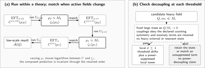
Sequential threshold evolution is an alternation, not one continuous beta function. Panel (a) evolves coefficients with $U_{n+2}$, matches with $\zeta_2$ near $M_2$, evolves with $U_{n+1}$, matches with $\zeta_1$ near $M_1$, and finally evolves to the observable scale; dependence on the arbitrary matching scales $\mu_i$ cancels through the retained order. Panel (b) checks the hierarchy, heavy-mass limit, coupling counting, symmetry and anomaly terms, and external kinematics. Passing gives shifts of operators with dimension at most four plus an inverse-mass-suppressed local tower; failure requires retaining the state or matching an unsuppressed effect. The diagram is schematic and not to scale.

Matching validation record

A defensible nondecoupling claim records the limit path and closes on an observable. The chapter’s shared record applies unchanged:

Record	Declare before matching	Closure check
Matching object and external data	Amplitude, form factor, Green function, background vertex or functional action; external species, polarizations, momenta and projections	The chosen objects span every coefficient combination claimed
Kinematics and retained order	On- or off-shell conditions, exceptional limits, expansion variables, inverse-mass order and loop order	Full and EFT expressions are expanded in the same variables and compared through the same order
Fields and normalization	Field coordinates, kinetic normalization, masses, LSZ residues and finite field maps	Two-point functions and external residues agree, or an explicit field transformation relates them
Gauge and auxiliary sectors	Quantum and background gauge fixing, ghosts, BRST-exact sectors and anomaly assumptions	Gauge-parameter or auxiliary-sector dependence cancels in the final observable
Operator basis and redundancies	Generating or reduced basis, integration-by-parts, equation-of-motion, evanescent and contact sectors	A complete map to the target basis reproduces the same amplitudes or invariant correlators
Ultraviolet scheme and matching scale	Regulator, subtraction convention, finite counterterms and $\mu_m$	Scheme and $\mu_m$ dependence cancels against coefficient running and matrix elements through the retained order
Infrared prescription	Light masses or virtualities, infrared regulator, overlap or zero-bin subtraction and order of limits	Every common infrared pole and logarithm cancels in full minus EFT before a hard coefficient is read off
Threshold and decoupling assumptions	Active fields, heavy-mass origin, coupling scaling, threshold order and hierarchy among heavy scales	Sequential and one-step organizations agree to the claimed order where both are valid
Observable closure and uncertainty	Validation observable, input parameters, truncation estimate, numerical tolerance and fit covariance	Independent observables agree within the decomposed uncertainty and show the expected residual scaling

The last row prevents a common false positive. A coefficient that tends to a constant is only a candidate. Hold the measured low-energy inputs fixed, assemble coefficients with matrix elements, verify Ward identities and anomaly constraints, and show that the full-minus-EFT residual follows the first omitted power or loop order. Report matching, running, power, parametric, and numerical uncertainties separately, with correlations when the same input or omitted term affects more than one component.

Common pitfalls

Sending a mass to infinity without specifying its origin. The limits $M\to\infty$ at fixed $y$ and $y\to\infty$ at fixed $v$ are different paths. Compute the background derivative or coupling exponents before invoking decoupling.

Calling every unsuppressed parameter shift nondecoupling. Heavy contributions to vacuum energy, scalar masses, and marginal couplings can grow or remain logarithmic. Decide which low-energy quantities are inputs before testing a prediction.

Inferring physics from one Wilson coefficient. Coefficients depend on basis, scheme, and matching scale. The claim survives only if an observable, Ward identity, or anomaly functional retains the effect.

Removing an anomalous subset of fermions without its determinant remainder. A heavy mass does not erase anomaly data. Include the Wess–Zumino term or change the low-energy degrees of freedom.

Putting light cuts into a hard coefficient. Nonanalytic light-momentum or light-mass dependence belongs to EFT matrix elements. Recheck the infrared subtraction and the order of limits.

Exercises

An operator of dimension six has a coefficient proportional to $y^2/M^2$. Classify its heavy limit for fixed $y$ and for $y=M/v$ at fixed $v$.

Solution

For fixed $y$, $s_y=0$ and $\omega=2s_y-2=-2$, so the contribution decouples as $1/M^2$. For $y=M/v$, $s_y=1$ and $\omega=0$, so the coefficient approaches $1/v^2$. The second limit violates the bounded-coupling hypothesis and eventually leaves perturbation theory.

Derive the coefficient of $hF_{\mu\nu}F^{\mu\nu}$ from the inverse-coupling threshold and explain why the answer vanishes in the vectorlike limit.

Solution

Expand

$$\ln m_\Psi^2(v+h) =\ln m_\Psi^2(v)+2\kappa_\Psi\frac{h}{v}+O(h^2).$$

In the normalization $-\mathcal F^2/(4e^2)$, the field-dependent part is $N_cQ_\Psi^2\kappa_\Psi h\mathcal F^2/(24\pi^2v)$. Rescaling to the canonical photon field with $\mathcal F=eF$ multiplies it by $e^2=4\pi\alpha$, giving $\alpha N_cQ_\Psi^2\kappa_\Psi hF^2/(6\pi v)$. At fixed $y$ and $v$, $\kappa_\Psi\sim yv/(\sqrt2M)$, so the coefficient vanishes as $1/M$.

References

• Appelquist, Thomas, and J. Carazzone. “Infrared Singularities and Massive Fields.” Physical Review D 11, no. 10 (1975): 2856–2861. DOI
• D’Hoker, Eric, and Edward Farhi. “Decoupling a Fermion Whose Mass Is Generated by a Yukawa Coupling: The General Case.” Nuclear Physics B 248, no. 1 (1984): 59–76. DOI
• Kniehl, Bernd A., and Michael Spira. “Low-Energy Theorems in Higgs Physics.” Zeitschrift für Physik C 69, no. 1 (1995): 77–88. DOI; arXiv