Wess–Zumino and WZW Terms

A Wess–Zumino term is not, in general, the integral of a globally defined local density on spacetime. Its invariant meaning is an exponentiated phase obtained from one dimension higher—or, intrinsically, from differential-cohomology or gerbe holonomy. Independence of the auxiliary extension quantizes the normalized periods. Adding a sigma-model kinetic term produces the Wess–Zumino–Witten (WZW) model, while boundaries turn the phase into relative data that can carry anomaly inflow.

Required background. When Is a Topological Term Well Defined? supplies the exponentiated-action and period tests. Cosets and Nonlinear Realizations supplies group-valued fields and their Maurer–Cartan forms.

Helpful background. Wess–Zumino Consistency and Descent develops the local descent equations used below, while de Rham periods and torsion explain why differential forms alone do not retain every global phase.

A Wess–Zumino phase is defined one dimension higher

Let $\Sigma^d$ be a closed oriented spacetime, $X$ a sigma-model target, and

$$\phi:\Sigma\longrightarrow X$$

the field. Let $H\in\Omega^{d+1}(X)$ be closed. Suppose the pair $(\Sigma,\phi)$ admits an oriented extension: there are an oriented $(d+1)$-manifold $B$ and a map $\widetilde\phi:B\to X$ such that

$$\partial B=\Sigma, \qquad \left.\widetilde\phi\right|_{\Sigma}=\phi.$$

The extension formula defines

$$\mathcal W_H[\phi;B,\widetilde\phi] = \exp\!\left( i\int_B\widetilde\phi^{\,*}H \right).$$

The auxiliary boundary $\partial B=\Sigma$ in this construction is not yet a physical boundary of the $d$-dimensional theory. It is a device for defining the phase on a closed spacetime. The central question is whether different devices give the same answer.

Locally, $H=dC_d$ may turn the extension integral into $\int_\Sigma\phi^*C_d$. That does not make $C_d$ global: changing target patch can shift it by lower-degree descent data. The phase $\mathcal W_H$, not a chosen local primitive, is therefore the global object. This is the same local-versus-global distinction that appears in Chern–Simons transgression. Witten 1984, printed pp. 458–459, eqs. (12)–(15) gives the compact-group construction and its extension ambiguity.

Orientation is part of the definition. Reversing the spacetime and extension gives

$$\mathcal W_H[-\Sigma]=\mathcal W_H[\Sigma]^{-1} =\overline{\mathcal W_H[\Sigma]},$$

for a unit-modulus phase. This is a sign reversal of the Wess–Zumino coupling, not a claim that the theory is orientation-independent.

Two extensions impose the period condition

Take two extensions $(B_1,\widetilde\phi_1)$ and $(B_2,\widetilde\phi_2)$ of the same boundary field. Reverse the orientation of $B_2$ and glue:

$$Y=B_1\cup_{\Sigma}(-B_2).$$

The maps glue to $\Phi:Y\to X$, and the ratio of phases is

$$\frac{\mathcal W_H[\phi;B_1,\widetilde\phi_1]} {\mathcal W_H[\phi;B_2,\widetilde\phi_2]} = \exp\!\left(i\int_Y\Phi^*H\right).$$

For the normalized presentation used in the figure, write

$$H=2\pi k\,\Omega_{d+1}, \qquad S_i=2\pi k\int_{B_i}\widetilde\phi_i^{\,*}\Omega_{d+1}, \quad i=1,2.$$

The relevant admissible period set is

$$\Lambda_\Omega = \left\{ \int_Y\Phi^*\Omega_{d+1} \;\middle|\; (Y,\Phi)\ \text{arises from an admissible gluing} \right\}.$$

Exact extension independence means $k\lambda\in\mathbb Z$ for every $\lambda\in\Lambda_\Omega$. If the normalized periods are integral and the admissible set contains a unit period, this immediately forces $k\in\mathbb Z$.

The figure packages this argument geometrically. Read it from left to right: the boundary data agree, the second filling is orientation-reversed, the fillings become a closed cycle, and the phase ratio becomes a closed period.

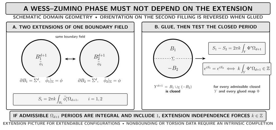
Two auxiliary fillings of the same boundary configuration produce the same Wess–Zumino phase exactly when their closed-period difference is invisible in the exponential. The diagram is schematic and assumes the configuration is extendable. Nonbounding sectors and torsion require an intrinsic differential completion.

Equivalently, the argument has four steps:

1. Fix the same oriented boundary field $(\Sigma,\phi)$ on both fillings.
2. Form the closed oriented $Y=B_1\cup_\Sigma(-B_2)$.
3. Evaluate the difference as the period $\int_Y\Phi^*H$.
4. Require that period to lie in $2\pi\mathbb Z$ for every admissible $(Y,\Phi)$.

A sufficient universal condition is

$$\left[\frac{H}{2\pi}\right]_{\mathrm{dR}} \in \operatorname{im}\!\left( H^{d+1}(X;\mathbb Z)\longrightarrow H_{\mathrm{dR}}^{d+1}(X) \right).$$

In the normalized presentation $H=2\pi k\,\Omega_{d+1}$, the cohomological condition is

$$k[\Omega_{d+1}]_{\mathrm{dR}} \in \operatorname{im}\!\left( H^{d+1}(X;\mathbb Z)\longrightarrow H_{\mathrm{dR}}^{d+1}(X) \right).$$

If $[\Omega_{d+1}]$ is the image of a primitive integral class and an admissible gluing realizes period one—as in the $SU(2)$ bubble test below—then both the universal cohomological test and the admissible-gluing test reduce to $k\in\mathbb Z$. More generally, if $[\Omega_{d+1}]=m[\Omega_{\mathrm{prim}}]$ with $m\in\mathbb Z$, $[\Omega_{\mathrm{prim}}]$ primitive integral, and an admissible gluing realizing its unit period, the tests reduce to $mk\in\mathbb Z$. Quantization is thus a statement about a coefficient, a normalized integral class, and the cycles actually admitted by the theory.

Nonbounding fields require intrinsic global data

The extension formula has two logically distinct requirements:

• an extension must exist; and
• the answer must be independent of which extension is chosen.

The first requirement is not automatic. Even if $\Sigma$ bounds as a bare oriented manifold, the map $\phi:\Sigma\to X$ need not extend. In oriented language, the decorated cycle $(\Sigma,\phi)$ must vanish in $\Omega_d^{\mathrm{SO}}(X)$. The familiar filling formula therefore gives a calculation on extendable configurations, not an intrinsic definition on every field sector.

An intrinsic completion replaces the differential form alone by a differential class

$$\widehat h\in\widehat H^{d+1}(X;\mathbb Z).$$

Its curvature records $H/2\pi$, while its holonomy assigns a phase directly to closed $d$-cycles. Flat and torsion data can change that holonomy without changing the curvature form, so an exact or even vanishing de Rham class does not by itself prove that every global Wess–Zumino phase is trivial. Davighi, Gripaios, and Randal-Williams 2023, § 3, arXiv v2, printed pp. 7–9 formulate topological actions as differential-cohomology pairings and make this global ceiling explicit.

For the concrete $SU(2)$ example below, the extension does exist because $\pi_2(SU(2))=0$. That special fact should not be promoted to a statement about arbitrary targets or spacetime dimensions.

The variation is local even when the action is not

Although the action itself may need an extension, its infinitesimal variation is intrinsic to $\Sigma$. Let $v$ be the variation vector along $\phi$, extended over $B$. Closedness of $H$, Cartan’s formula, and Stokes’ theorem give

$$\begin{aligned} \delta_v S_{\mathrm{WZ}} &= \int_B\widetilde\phi^{\,*}\mathcal L_v H \\ &= \int_B\widetilde\phi^{\,*}d(\iota_v H) \\ &= \int_\Sigma\phi^*(\iota_v H). \end{aligned}$$

Suppose vector fields $v_a$ generate a symmetry and locally

$$\iota_{v_a}H=d\mu_a.$$

For a spacetime-dependent parameter $\epsilon^a$, the closed-spacetime variation becomes

$$\delta_\epsilon S_{\mathrm{WZ}} = -\int_\Sigma d\epsilon^a\wedge\phi^*\mu_a.$$

Constant parameters therefore give the expected global invariance in this local presentation. Gauging asks for more: the invariant differential class must admit compatible equivariant data on every overlap and higher overlap. Failure of that lift is an obstruction, while the displayed variation captures only its local descent shadow. Torsion and other global anomalies are not decided by this formula alone. Davighi, Gripaios, and Randal-Williams 2023, § 8, arXiv v2, printed pp. 27–30 give the equivariant-to-invariant comparison and its gauging interpretation.

First application: the SU(2) WZW phase in the topological-action thread

Take a closed oriented Euclidean worldsheet $\Sigma=S^2$ and a field

$$g:\Sigma\longrightarrow SU(2)\simeq S^3.$$

Write

$$\vartheta=g^{-1}dg$$

for the anti-Hermitian Maurer–Cartan form and $\operatorname{Tr}_{\mathrm f}$ for the fundamental trace. This is a group-valued-field convention, translated explicitly from the site’s Hermitian gauge-potential convention. Choose the target orientation so that

$$\eta_3 = \frac{1}{24\pi^2} \operatorname{Tr}_{\mathrm f} \bigl(\vartheta\wedge\vartheta\wedge\vartheta\bigr), \qquad \int_{SU(2)}\eta_3=1.$$

Because $\pi_2(SU(2))=0$, every such $g$ extends to $\widetilde g:B^3\to SU(2)$. Define

$$\mathcal W_k[g;\widetilde g] = \exp\!\left( 2\pi i k\int_{B^3}\widetilde g^{\,*}\eta_3 \right).$$

A degree-n bubble detects the level

Choose the boundary field $g$ to be constant. One filling is constant. Another agrees at the boundary but contains an interior bubble

$$q_n:B^3\longrightarrow SU(2)$$

that is constant on $\partial B^3$. Collapsing the boundary identifies $B^3/\partial B^3\simeq S^3$, so $q_n$ has any chosen degree $n\in\mathbb Z$. The two extensions differ by

$$\Delta S_{\mathrm{WZ}} = 2\pi k\int_{S^3}q_n^*\eta_3 = 2\pi kn.$$

Their phase ratio is $e^{2\pi i kn}$. Every degree is invisible precisely when

$$k\in\mathbb Z.$$

This proves integer level in the declared primitive normalization. It does not derive an integer merely from the notation $k$, nor does it classify non-simply-connected or spin-refined WZW models. Witten 1984, printed pp. 458–459, eqs. (12)–(15) gives the original extension and winding-number argument.

Adding the kinetic term gives the WZW model

The Wess–Zumino phase is metric-independent, but the full WZW model also contains a kinetic term. For positive $k$, one Euclidean convention is

$$S_{\mathrm{kin}}[g] = -\frac{k}{8\pi} \int_\Sigma \operatorname{Tr}_{\mathrm f} \bigl(\vartheta\wedge *\vartheta\bigr) \ge 0,$$

and

$$e^{-S_E[g]} = e^{-S_{\mathrm{kin}}[g]}\, \mathcal W_k[g;\widetilde g].$$

Equivalently,

$$S_E = S_{\mathrm{kin}} -2\pi i k\int_{B^3}\widetilde g^{\,*}\eta_3 \quad \pmod{2\pi i}.$$

The Hodge star belongs only to the kinetic term. A generic sigma model with a quantized Wess–Zumino phase need not sit at the conformal WZW coupling; affine current algebra, the Sugawara stress tensor, integrable representations, and Knizhnik–Zamolodchikov equations require additional dynamics.

The four-model thread compares tests, not theories

A topological quantum field theory (TQFT) is a dynamical field theory with topological gluing and state-space data. The label does not follow merely from a metric-independent phase. The table compares the global-definition test across this page and the preceding Chern–Simons, BF, and finite-gauge examples. The rows are not equivalent theories.

Shared global-action tests across four models; the rows are comparisons, not equivalences.

Model and field role	Global defining datum	Coefficient or label test	Boundary or dynamical consequence	Stop condition
WZ/WZW sigma-model field	Map to a target with an integral differential class	Closed-period independence; integer k only in a primitive normalization	A physical boundary needs a gerbe trivialization; the WZW kinetic term remains metric-dependent	Not an Abelian gauge TQFT and no BF or finite-gauge state count follows
Compact U(1) Chern–Simons	Compact connection and differential characteristic class	One-component bosonic level even; spin level integral in the stated normalization	Fixed connection gives a response; integrating it gives a dynamical TQFT; a boundary needs a polarization or completion	The Abelian boundary mode is not the SU(2) cubic Wess–Zumino volume term
Compact BF	Compact gauge fields with integral flux and pairing	Large-gauge invariance makes the pairing level integral	Fixed fields give a cross-response; summing both gives the finite gauge TQFT	Boundary modes and state spaces depend on the compact global data and boundary condition
Finite Dijkgraaf–Witten theory	Finite bundle and a group-cohomology class	Cocycle class is discrete; no differential-form extension is required	A fixed bundle gives a phase; the automorphism-weighted bundle sum defines the dynamical theory	Do not identify the cocycle evaluation with a sigma-model Wess–Zumino density

For compact Abelian Chern–Simons theory, the spin-versus-bosonic level lattice is the extension test in a differential-character normalization Belov and Moore 2005, §§ 1–2, arXiv v1, printed pp. 3–8. Compact BF requires its global Deligne–Beilinson data and integer pairing Kapustin and Seiberg 2014, § 3, arXiv v2, printed pp. 9–13, eqs. (3.1)–(3.16). A finite Dijkgraaf–Witten weight is a cocycle evaluation, whereas the dynamical theory uses a bundle sum Dijkgraaf and Witten 1990, §§ 6.2 and 6.4, printed pp. 415–416 and 420–423; Freed and Quinn 1993, §§ 1–2, printed pp. 438–445 supply the groupoid-weighted measure and boundary-line interpretation.

Chern–Simons inflow produces a chiral boundary theory

There is a precise non-Abelian relation between Chern–Simons and WZW data, but it needs boundary choices. In an anti-Hermitian convention, write

$$S_{\mathrm{CS}}[A] = \frac{k}{4\pi} \int_M \operatorname{Tr} \left( A\wedge dA+\frac{2}{3}A\wedge A\wedge A \right).$$

On a three-manifold with boundary, an infinitesimal gauge transformation gives

$$\delta_\epsilon S_{\mathrm{CS}} = \frac{k}{4\pi} \int_{\partial M} \operatorname{Tr}(\epsilon\,dA),$$

up to the sign fixed by the induced-boundary and gauge-action conventions. The choice of boundary counterterm can change the displayed consistent representative. The bulk phase is therefore relative to boundary data rather than a gauge-invariant number by itself.

Choose an admissible boundary condition and polarization. The bulk equation $F=0$ can then be solved locally as

$$A=-dU\,U^{-1}.$$

Substitution into the boundary-reduced action produces a chiral WZW action at the same level. A different polarization changes which chirality is exposed, and the nonchiral $G_L\times G_R$ model naturally pairs with a difference $S_{\mathrm{CS}}[A_L]-S_{\mathrm{CS}}[A_R]$. None of this says that an unqualified Chern–Simons boundary automatically carries the full nonchiral WZW model. Elitzur, Moore, Schwimmer, and Seiberg 1989, § 2, author-preprint printed pp. 3–5, eqs. (2.2)–(2.8) derive the boundary variation, flat-connection reduction, and chiral action.

For $U(1)$, the cubic group form $\operatorname{Tr}(g^{-1}dg)^3$ vanishes. The familiar Abelian Chern–Simons boundary chiral boson is consequently not a literal $U(1)$ version of the $SU(2)$ volume-form construction above. Abelian Chern–Simons belongs in the comparison because it obeys a parallel global phase test, not because the local theories are the same.

A physical boundary needs a trivialization

Now let the $d$-dimensional spacetime itself have a physical boundary. The closed-spacetime Wess–Zumino amplitude is no longer canonically a number. It is naturally a vector in a line over the boundary field, and a boundary condition must trivialize that line.

One geometric realization chooses a brane submanifold $Q\subset X$ on which the boundary field lands and a two-form $\omega$ satisfying, in the two-dimensional WZW case,

$$\left.H\right|_Q=d\omega.$$

If a surface $D\subset Q$ caps the physical boundary and $\partial B=\Sigma\cup(-D)$, a relative representative is

$$\exp\!\left( i\int_B\widetilde\phi^{\,*}H -i\int_D\phi_Q^*\omega \right),$$

with signs fixed by the displayed orientation convention. Consistency still requires integral relative periods. More general boundaries can require Chan–Paton or module data in addition to this elementary trivialization. Gawędzki and Reis 2002, § 2.2, printed pp. 5–6, eqs. (2.7)–(2.16), and § 7, printed pp. 22–23, eqs. (7.1)–(7.6) distinguish the scalar closed-worldsheet amplitude from the line-valued boundary amplitude and construct the brane trivialization.

This physical boundary is distinct from the auxiliary $\partial B=\Sigma$ used to define a closed-worldsheet phase, and both are distinct from the three-dimensional Chern–Simons bulk whose boundary supports an inflow-canceling chiral theory.

What the extension test does not prove

The period calculation is powerful but deliberately narrow.

• It does not prove conformal invariance. Quantizing the Wess–Zumino phase does not tune the sigma-model metric to the WZW fixed point.
• It does not prove gaugeability. An invariant class may fail to admit the equivariant differential lift required for gauging.
• It does not see every global phase. Differential forms omit flat torsion data, and a filling formula omits nonbounding field configurations until it is intrinsically completed.
• It does not classify boundaries. A brane trivialization is one input; consistent boundary operator spectra and sewing data require more.
• It does not make the WZW model a TQFT. The kinetic term depends on the worldsheet metric even though the Wess–Zumino factor is topological.
• It does not fix current algebra or spectra. Those depend on the full conformal dynamics, representation theory, and global form of the target.

For non-simply-connected targets, the allowed levels can form a proper sublattice and can carry extra discrete choices. Spin variants may alter the level data; unorientable worldsheets require orientation-twisted structures rather than the oriented formula above. These are changes of the global problem, not corrections to the $SU(2)$ primitive-period calculation.

Common pitfalls

Assuming every map extends. A bare spacetime may bound while the decorated cycle $(\Sigma,\phi)$ does not. Use the filling formula only after checking extension existence, or define the phase intrinsically.

Calling closedness quantization. The equation $dH=0$ makes the infinitesimal variation a boundary term; integral periods make the exponentiated action independent of the filling. These are different tests.

Calling every Wess–Zumino coefficient an integer. Integer $k$ follows in the displayed $SU(2)$ primitive normalization. A nonprimitive generator, quotient target, or refined tangential structure changes the coefficient lattice.

Confusing three boundaries. The auxiliary filling boundary, a physical worldsheet boundary, and a Chern–Simons inflow boundary play different roles and require different data.

Equating Abelian Chern–Simons with the $SU(2)$ WZW volume term. Their global quantization tests are comparable, but the Abelian cubic Maurer–Cartan form vanishes and the boundary reductions are not identical local constructions.

Check your understanding

1. Recover the two-filling condition. Starting from two extensions, show that their phase ratio is a closed period.

Solution

Reverse the orientation of $B_2$, glue along the common $(\Sigma,\phi)$, and call the resulting map $\Phi:Y\to X$. Additivity and orientation reversal give

$$\int_{B_1}\widetilde\phi_1^*H - \int_{B_2}\widetilde\phi_2^*H = \int_Y\Phi^*H.$$

Exponentiating gives the displayed phase ratio. It equals one for every admissible gluing exactly when every such period lies in $2\pi\mathbb Z$.

2. Test a half-integral $SU(2)$ level. What happens at $k=1/2$ for a degree-one interior bubble?

Solution

The phase ratio is

$$e^{2\pi i k}=e^{\pi i}=-1.$$

The same boundary field receives two different amplitudes, so the proposed phase is not extension-independent in this normalization.

3. Change the normalization. Suppose $\Omega=2\Omega_{\mathrm{prim}}$, where $[\Omega_{\mathrm{prim}}]$ is a primitive integral class and an admissible gluing realizes its unit period. What does extension independence require?

Solution

Every admissible closed period of $\Omega$ is an even integer, and the stated unit-period gluing for $\Omega_{\mathrm{prim}}$ realizes the value two. Thus

$$e^{2\pi i k\int_Y\Omega}=1$$

for every admissible gluing precisely when $2k\in\mathbb Z$. A half-integral $k$ is then allowed. This is why the class normalization must accompany any level statement.

4. Reverse orientation. What happens to the Wess–Zumino factor?

Solution

The extension integral changes sign, so the unit phase is inverted:

$$\mathcal W_H[-\Sigma]=\mathcal W_H[\Sigma]^{-1}.$$

For a unitary phase this is complex conjugation. It does not remove the need to specify an orientation.

5. Distinguish the WZ term from the WZW model. Which part uses the worldsheet metric?

Solution

The extension phase depends on orientation and global target data but not on a worldsheet metric. The kinetic term contains the Hodge star and is metric-dependent. The full WZW model contains both.

6. Diagnose a physical boundary. Why is the bulk extension integral alone insufficient when $\partial\Sigma\ne\varnothing$?

Solution

The Wess–Zumino amplitude is then line-valued over the boundary field rather than canonically scalar. A brane support and trivialization—represented locally by $H|_Q=d\omega$ and the compensating boundary integral—are needed before a number is assigned.

Continue to current algebra and topological models

For conformal dynamics, Affine Current Algebras and WZW Models will develop the current OPE, Sugawara construction, integrable representations, and KZ equations.

For the neighboring topological theories, Chern–Simons Actions and Level Quantization gives the full global level and framing analysis, while BF Couplings and Discrete Topological Data will develop the compact BF and finite-gauge thread. Wess–Zumino Consistency and Descent is the place to continue the local anomaly calculation.

Intrinsic differential characters, bordism refinements, generalized cohomology, and the classification of equivariant lifts belong to a theorem-first Mathematical QFT treatment. This page uses their consequences only to state the global ceiling of the extension formula.

References

• Dmitriy M. Belov and Gregory W. Moore, “Classification of Abelian Spin Chern–Simons Theories,” arXiv:hep-th/0505235v1 (2005). Stable record.
• Joe Davighi, Ben Gripaios, and Oscar Randal-Williams, “Differential Cohomology and Topological Actions in Physics,” Advances in Theoretical and Mathematical Physics 27.7 (2023), 2045–2085. DOI. Open PDF, arXiv:2011.05768v2.
• Robbert Dijkgraaf and Edward Witten, “Topological Gauge Theories and Group Cohomology,” Communications in Mathematical Physics 129 (1990), 393–429. DOI.
• Shmuel Elitzur, Gregory Moore, Adam Schwimmer, and Nathan Seiberg, “Remarks on the Canonical Quantization of the Chern–Simons–Witten Theory,” Nuclear Physics B 326.1 (1989), 108–134. DOI. Open author PDF.
• Daniel S. Freed and Frank Quinn, “Chern–Simons Theory with Finite Gauge Group,” Communications in Mathematical Physics 156 (1993), 435–472. DOI. Open PDF, arXiv:hep-th/9111004v3.
• Krzysztof Gawędzki and Nuno Reis, “WZW Branes and Gerbes,” Reviews in Mathematical Physics 14.12 (2002), 1281–1334. DOI. Open PDF, arXiv:hep-th/0205233.
• Anton Kapustin and Nathan Seiberg, “Coupling a QFT to a TQFT and Duality,” Journal of High Energy Physics 2014.4 (2014), article 001. DOI. Open PDF, arXiv:1401.0740v2.
• Edward Witten, “Non-Abelian Bosonization in Two Dimensions,” Communications in Mathematical Physics 92 (1984), 455–472. DOI. Open PDF.