

Support, Codimension, and Operator Data
An operator supported on a curve, surface, wall, or boundary is not specified by its support alone. A complete definition records the embedded or stratified support, its normal and transverse data, any orientation, coorientation, or framing, the operator label and global gauge data, endpoint and junction rules, renormalization, and the class of deformations under which the insertion is meant to be invariant. Two insertions can occupy the same submanifold and still be different operators.
Codimension remains the first useful organizing datum because it determines the local transverse problem. It does not determine whether an insertion is geometric or topological, genuine or attached, a symmetry defect or a general defect, nor whether it can end or fuse. Those are additional parts of the definition.
Required background. Local and Composite Operator Insertions supplies the regulated meaning of an insertion, its labels, and the need for operator renormalization.
Helpful background. Differential Forms, Integration, Orientation, and Stokes Theorem supplies pullback, orientation, induced boundary orientation, and transverse flux integration.
Codimension organizes the transverse problem
Section titled “Codimension organizes the transverse problem”Work first in Euclidean signature and let a smooth interior stratum be an embedding
Here is the support dimension and is its codimension. Along the support, tangent and normal directions fit into
At a smooth interior point , a sufficiently small tubular neighborhood has a normal disk . Its boundary is the local transverse link
Globally these links form the sphere bundle . It is generally not a product : the normal bundle can twist. This local slice and normal-bundle statement follows from Lee 2013, 2nd ed., Ch. 5, p. 99 and pp. 106–107, Prop. 5.16. After choosing a Riemannian metric on , the normal exponential map supplies the arbitrary-manifold tubular neighborhood used here Lee 2018, 2nd ed., § 5, pp. 133–135, especially eq. (5.21) and Thm. 5.25.
Orientation data should be stated rather than inferred. One useful normal-first convention is
When the relevant orientations exist, any two of the ambient, tangent, and normal orientations determine the third. The normal orientation in turn orients each linking sphere. A framing is stronger: it is a trivialization of , normally used through its homotopy class. It need not exist, and it is required only when the operator definition is framing-sensitive.
The smooth-interior hypothesis matters. A codimension-one internal interface has local link , whose two points record its two sides. A spacetime boundary instead has a one-sided collar , not a full link Lee 2013, 2nd ed., Ch. 9, pp. 222–223, Thm. 9.25. At an endpoint, corner, intersection, or junction, the support is stratified and the link is decorated by the incident strata; the plain sphere formula no longer gives the whole local model.
Support geometry does not determine operator type
Section titled “Support geometry does not determine operator type”In Euclidean functional-integral language, “operator,” “observable,” and “defect” are often used with overlapping meanings. A positive-dimensional insertion is commonly called an extended operator or a defect, while a time-slice operator and its time-extended history need not be described by the same word. What matters is to declare the convention and the data, not to force every author’s terminology into disjoint boxes Gaiotto, Kapustin, Seiberg, and Willett 2015, Introduction, arXiv v2, pp. 1–3, especially eqs. (1.1)–(1.2), Open PDF.
The following distinctions are operational:
-
A local insertion has point support. Its field label and renormalized definition remain essential even though its geometry is simple.
-
An extended operator or defect has positive-dimensional support or changes the field-theory data across a locus. The terms overlap in common usage.
-
An interface is an interior codimension-one defect with two bulk sides. A boundary is part of the spacetime domain and has only one bulk side.
-
A topological defect is invariant under a declared class of structure-preserving deformations that avoid forbidden crossings and carry all attached strata with it. Positive-dimensional support alone does not imply this invariance.
-
A symmetry defect is equipped with an action on charged insertions and with fusion and junction data. For an ordinary group symmetry it is invertible and topological; more general topological defects need not be group-like.
-
An endpoint or junction is a lower-dimensional stratum with its own allowed operator. A conservation equation for labels is necessary data, not a proof that the junction exists.
Topological symmetry operators and their actions are developed with these precise deformation and fusion conditions in Bhardwaj et al. 2024, § 2.1, arXiv v2, pp. 6–9, Statement 2.1 and eqs. (2.4)–(2.23); § 2.2.1, pp. 12–14, Definition 2.1 and eqs. (2.38)–(2.45), Open PDF.
The atlas below separates the local transverse classification from the quantum data. Inspect the interface and boundary cards first, then the bottom rule: the same value of and does not supply side assignments, labels, attachments, renormalization, or deformation laws.
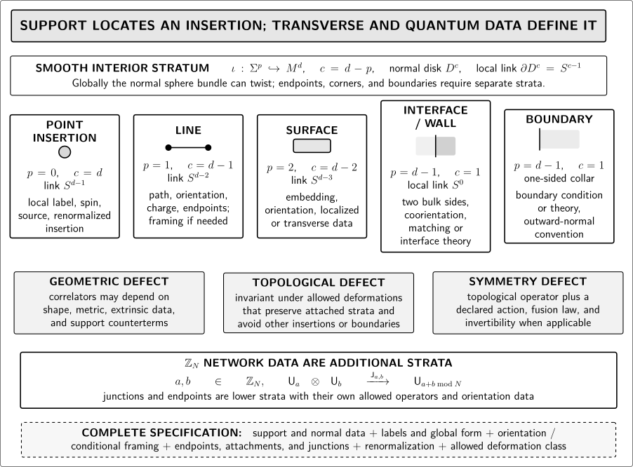
For a smooth interior support , codimension gives the local normal disk and link . The atlas also records the one-sided boundary exception and a finite-symmetry junction. It is a schematic, not-to-scale classification: the normal sphere bundle can twist, and endpoints, corners, and junctions require stratified data.
| Object or stratum | Support and transverse model | Additional defining data | What geometry alone does not imply |
|---|---|---|---|
| Point insertion | p = 0; local link S^(d−1) | Field or composite label, spin, source, normalization, regulator | Gauge invariance, primarity, or a regulator-independent product |
| Line | p = 1; local link S^(d−2) | Path, orientation, charge or representation, endpoints, optional framing | Genuineness, topological invariance, or permission to end |
| Surface | p = 2; local link S^(d−3) | Embedding, orientation, transverse singularity or defect-local theory | Invertibility, symmetry action, or shape independence |
| Interior interface | p = d−1; local S⁰ with two sides | Ordered bulk theories, coorientation, matching conditions, interface fields | A one-sided boundary condition or an invertible wall |
| Boundary | p = d−1; one-sided collar | Boundary condition or boundary theory, outward normal, allowed transformations | A second bulk side or the full S⁰ interface model |
| Symmetry defect | For a 0-form symmetry, a codimension-one topological sheet | Group label, action on charges, fusion, orientation, junctions | That every topological defect is invertible or group-like |
| Endpoint or junction | Lower stratum with a decorated, generally non-spherical link | Incidence and orientation convention, allowed junction operator, coherence | Existence from label conservation alone |
A complete operator record is a data sheet
Section titled “A complete operator record is a data sheet”Before manipulating an extended insertion, record the applicable entries below. “Applicable” matters: not every operator needs an orientation, framing, singularity, or endpoint.
-
Ambient theory and background. Specify the QFT, spacetime domain, metric or tangential structure, gauge-group global form, and boundary conditions.
-
Support. Give the embedding or stratification, its dimension and codimension, and whether it is closed, open, knotted, linked, or incident on other strata.
-
Normal data. State the local link or transverse boundary condition, together with tangent and normal orientations, a coorientation, and a framing only when required.
-
Quantum label. Supply the charge, representation, group element, monodromy, boundary condition, defect-local theory, or coupling that distinguishes the insertion.
-
Attachments. List endpoint fields, attached lines or surfaces, crossing rules, junction maps, and the orientations used in their incidence equations.
-
Global and genuine status. Say whether the insertion is defined on every allowed bundle, whether it requires an attached higher-dimensional operator, and which dynamical objects can screen or terminate it.
-
Renormalized definition. State the regulator, normalization, and support, cusp, corner, or junction counterterms needed to define its correlators.
-
Deformation law. Declare whether correlators may depend on the precise embedding, only on an isotopy or framed-isotopy class, or only on topology and linking subject to stated exclusions.
This data sheet prevents a common category error: “a line” is a support type, not an operator type.
One curve can support inequivalent Abelian line operators
Section titled “One curve can support inequivalent Abelian line operators”Consider compact gauge theory on an oriented Euclidean four-manifold. Let be the faithfully normalized compact connection,
for every closed oriented two-cycle . A closed oriented curve carries the electric Wilson line
Its support has , , and local transverse link . Reversing the curve reverses the holonomy,
The curve and the integer label are both necessary. In a non-Abelian theory the corresponding label is a representation, and orientation reversal conjugates it Witten 1989, § 1, pp. 355–356, eq. (1.5).
On an open path ,
If a field has charge , the dressed insertion
is gauge invariant. Without suitable endpoint operators, boundary data, or an attached defect, the open Wilson line is not a genuine insertion. This endpoint cancellation, translated to the convention above, is worked out in Bhardwaj et al. 2024, § 3.2.1, arXiv v2, p. 29, Definition 3.2 and eqs. (3.11)–(3.15), Open PDF.
The same curve can instead support a magnetic disorder line. Its defining datum is not the Wilson holonomy but the flux through each sufficiently small oriented linking sphere:
The equivalent singular boundary behavior and its flux normalization are given in Kapustin 2006, § 3.2, arXiv v3, pp. 10–11, especially the boundary condition immediately before eq. (3.6), Open PDF.
Thus the electric and magnetic lines have identical support dimension, codimension, and local link, yet different transverse definitions. A full construction must say how the gauge field is singular, which global form and charge lattice are allowed, and whether an attached surface is physical. Those issues continue in Disorder Operators and Singular Boundary Conditions.
Nothing in either support specification proves topological invariance. An ordinary Maxwell Wilson line is a geometric, renormalized insertion; its correlators can depend on shape, metric, and support counterterms. Likewise, charge quantization does not by itself make the magnetic line topological.
A finite symmetry network needs junction operators
Section titled “A finite symmetry network needs junction operators”Now consider a three-dimensional QFT with a non-anomalous zero-form symmetry . Its group-like symmetry defects are topological surfaces labeled by . They have , , and the two-sided local link . Reversing their coorientation inverts the label:
When the sheet is swept across a local operator of charge , it supplies the phase
Two incoming sheets can fuse to an outgoing sheet along a line junction:
With two incoming labels and one outgoing label , the declared orientation convention gives
This equation does not construct . Its existence, normalization, defect-local degrees of freedom, and compatibility where several line junctions meet are extra data. Nor may a sheet simply end in empty bulk: an endpoint line must be among the allowed strata. Flat finite-symmetry backgrounds as networks of codimension-one defects and higher-codimension junctions are described in Gaiotto, Kapustin, Seiberg, and Willett 2015, § 2, arXiv v2, pp. 6–7, especially the group law in eq. (2.2), action in eqs. (2.3)–(2.4), and the defect-network paragraph on p. 7, Open PDF. The phase and additive fusion above are those formulas specialized to ; the junction map itself is additional data. A nontrivial anomaly can obstruct an ordinary coherent network, which is why the non-anomalous hypothesis was stated at the outset.
The line junction, surface sheets, and local charged operator form a stratified network. Their dimensions alone do not specify their fusion or action.
Topological, geometric, and framed are independent properties
Section titled “Topological, geometric, and framed are independent properties”Let be a family of embeddings that preserves every declared tangential, normal, attachment, and boundary condition. A topological defect passes the deformation test
whenever the isotopy avoids other insertions and physical boundaries except through specified crossing or endpoint rules. Even then, the correlator can depend on topology, linking, orientation, labels, and—if declared—framing. In conformal defect theory, the displacement operator measures the response to transverse shape deformations, providing a useful model-specific diagnostic rather than a definition for all QFT defects Billò et al. 2016, Introduction, arXiv v2, pp. 2–3, eqs. (1.1)–(1.4); § 5.1, pp. 27–31, eqs. (5.1)–(5.25), Open PDF.
Framing is a separate question. Three-dimensional Chern–Simons Wilson loops provide the standard bounded example: regulating self-linking requires a knot framing, and changing that framing changes the quantum phase Witten 1989, § 2.1, pp. 362–365, especially Fig. 3 and eqs. (2.29)–(2.33). This example does not license the statement that every line in every QFT is framed. A framing must be required by the operator’s definition or regularization, and a chosen framing restricts the allowed deformations to framing-preserving ones.
The next canonical example is Wilson Lines and Loops, where parallel transport, representation labels, genuineness, framing, and renormalization are developed together. Fusion, Junctions, and Endpoints develops network composition. For theorem-level stratified composition and higher morphisms, see Defects on Stratified Spacetimes and Higher-Categorical Composition.
Common pitfalls
Section titled “Common pitfalls”Codimension names the operator. Codimension fixes a local transverse dimension, not a charge, representation, singularity, boundary condition, or fusion law. Wilson and magnetic lines on the same curve are the elementary counterexample.
A boundary is just an interface with one theory deleted. An interior interface has a two-sided normal model and data on both sides. A boundary is part of the spacetime domain, has a one-sided collar, and requires a boundary condition or boundary theory.
Every extended operator is topological. Topological status is a deformation-invariance statement about correlators in a specified domain. Generic Wilson lines, conformal defects, and interfaces can retain geometric and renormalization dependence.
Every line needs a framing. Orientation and framing are different. Framing is a trivialization of the normal bundle and is included only when the definition or regularization requires it.
An open Wilson line is automatically gauge invariant. Its endpoint variation is nonzero. Endpoint fields, boundary data, or an attached defect must cancel that variation.
Check your understanding
Section titled “Check your understanding”1. Links in four dimensions
Section titled “1. Links in four dimensions”For a point, line, surface, and internal wall in , find and the local link. Why is the answer for a spacetime boundary different?
Solution
The point has and link ; the line has and ; the surface has and ; the internal wall has and . A spacetime boundary also has dimension three and codimension one, but it has a one-sided collar rather than the two-sided model of an interior wall.
2. Two lines on one curve
Section titled “2. Two lines on one curve”On the same closed curve in compact four-dimensional gauge theory, compare the data defining an electric Wilson line of charge and a magnetic line of charge .
Solution
Both have , , and a small link. The Wilson line is defined by the connection holonomy and the integer electric label . The magnetic line is defined by the transverse boundary condition . Equal supports and links therefore do not make the operators equal.
3. Dress an open Wilson line
Section titled “3. Dress an open Wilson line”Let and let transform as . Verify that is gauge invariant.
Solution
The three factors acquire , , and . Their product is one. Removing either endpoint field leaves an uncancelled gauge variation.
4. Read a finite-symmetry junction
Section titled “4. Read a finite-symmetry junction”For , two incoming sheets have labels and . What is the outgoing label in the convention above? Does the label equation prove that a junction exists?
Solution
The outgoing label is . The equation is only the incidence or conservation rule. One must still specify an allowed junction operator , its normalization and local degrees of freedom, and its compatibility with other junctions.
5. Test the word “topological”
Section titled “5. Test the word “topological””An author calls a line topological because its charge is quantized. What must be checked instead?
Solution
One must vary the embedding through the declared class of allowed isotopies, carry all endpoint and junction strata with it, avoid forbidden crossings and boundaries, and check that correlators do not change. Quantized charge alone does not establish this. If the line is framing-sensitive, the comparison must also preserve the chosen framing.
References
Section titled “References”-
Bhardwaj, Lakshya, Lea E. Bottini, Ludovic Fraser-Taliente, Liam Gladden, Dewi S. W. Gould, Arthur Platschorre, and Hannah Tillim. “Lectures on Generalized Symmetries.” Physics Reports 1051 (2024): 1–87. DOI. Open PDF, arXiv v2.
-
Billò, Marco, Vasco Gonçalves, Edoardo Lauria, and Marco Meineri. “Defects in Conformal Field Theory.” Journal of High Energy Physics 2016, no. 4 (2016): 091. DOI. Open PDF, arXiv v2.
-
Gaiotto, Davide, Anton Kapustin, Nathan Seiberg, and Brian Willett. “Generalized Global Symmetries.” Journal of High Energy Physics 2015, no. 2 (2015): 172. DOI. Open PDF, arXiv v2.
-
Kapustin, Anton. “Wilson–’t Hooft Operators in Four-Dimensional Gauge Theories and S-Duality.” Physical Review D 74, no. 2 (2006): 025005. DOI. Open PDF, arXiv v3.
-
Lee, John M. Introduction to Smooth Manifolds. 2nd ed. Graduate Texts in Mathematics 218. New York: Springer, 2013. DOI. Author corrections, updated 3 January 2026.
-
Lee, John M. Introduction to Riemannian Manifolds. 2nd ed. Graduate Texts in Mathematics 176. Cham: Springer, 2018. DOI.
-
Witten, Edward. “Quantum Field Theory and the Jones Polynomial.” Communications in Mathematical Physics 121, no. 3 (1989): 351–399. DOI. Open PDF.
Original QFT.org content:CC BY 4.0, unless an item supplies different terms. Third-party material retains its own terms.