Abelian Chern–Simons Theory

For a compact bosonic Abelian Chern–Simons theory with an even, nonsingular symmetric integral matrix $K$, the finite line content is the discriminant group

$$\mathcal A=\mathbb Z^r/K\mathbb Z^r.$$

Fusion is addition in $\mathcal A$, the inverse matrix $K^{-1}$ determines mutual braiding, and—when $K$ is even—the associated quadratic refinement determines topological spin. On a closed genus-$g$ surface the state-space dimension is $\lvert\det K\rvert^g$. These formulas answer the line-operator and finite-state questions, but only after the compact charge lattice, orientation, spin or non-spin structure, framing convention, and boundary conditions have been declared. They do not by themselves classify all Abelian topological phases.

Unless stated otherwise, this page begins with a closed smooth oriented three-manifold, compact gauge torus $U(1)^r$, a chosen quantum framing or equivalent relative gravitational convention, and an even, nonsingular integral $K$. “Even” means $n^{\mathsf T}Kn\in2\mathbb Z$ for every $n\in\mathbb Z^r$, equivalently that every diagonal entry is even. Odd integral $K$ defines a spin theory and requires the separate refinements described below.

Required background. Chern–Simons Actions and Level Quantization supplies the global phase, compact-field normalization, and bosonic-versus-spin level lattice. Linking, Braiding, and Framing separates a full braid from an exchange and explains why a self-twist needs a framing. Helpful background. State Spaces, Cobordisms, and Gluing provides the trace and surgery checks used for the finite state spaces below.

Compact Abelian Chern–Simons data and its domain

Let $a^I$, $I=1,\ldots,r$, be compact $U(1)$ connections. In a local trivialization the Lorentzian action is written

$$S_K[a] = \frac{1}{4\pi} \int_M K_{IJ}\,a^I\wedge da^J, \qquad K=K^{\mathsf T}.$$

This differential-form expression is shorthand for a globally defined differential-cohomological Chern–Simons phase. The $a^I$ need not be global one-forms, and treating them that way would erase the flux sectors that make the line quotient and finite Hilbert spaces possible.

For an ordinary oriented bosonic theory, the compact large-gauge test gives

$$K_{IJ}\in\mathbb Z, \qquad K_{II}\in2\mathbb Z.$$

A spin structure permits an arbitrary symmetric integral $K$, including odd diagonal entries. This is a change in tangential structure, not in orientation. Independently, quantizing the theory can introduce a three-manifold framing phase controlled here by the lattice signature. In the chosen positive convention, an $s$-unit framing change acts as

$$Z \longmapsto Z\, \exp\left( \frac{2\pi i\,s\,\operatorname{sign}(K)}{24} \right),$$

up to complex conjugation with the opposite orientation convention. The phase cancels when $\operatorname{sign}(K)=0$, as it does for the $BF$ matrix below. Spin does not in general remove framing dependence, and framing does not change the classical level lattice. This three-manifold framing anomaly is also distinct from the self-framing of an individual Wilson line used to define $\theta_\ell$. Witten derives the regulated framing law in Witten 1989, § 2, printed pp. 360–361, eqs. (2.18)–(2.25), Open PDF; the Abelian lattice formula is summarized in Belov and Moore 2005, § 5.6.1, printed p. 35, eq. (5.45), arXiv v1 PDF.

The nonsingularity condition

$$\det K\ne0$$

is essential for the finite formulas on this page. It makes the classical equation $K_{IJ}da^J=0$ imply local flatness and makes the induced pairing on line labels nondegenerate. If $\det K=0$, continuous zero modes remain and the finite discriminant-group description is not the claimed TQFT.

An integral change of gauge-field basis

$$a=W a', \qquad W\in GL(r,\mathbb Z),$$

gives

$$K'=W^{\mathsf T}KW.$$

This is an isomorphism of the compact charge lattice, not a new theory. A Wilson charge transforms as $\ell'=W^{\mathsf T}\ell$, and all formulas below are invariant under the simultaneous transformation. More general notions of stable equivalence, including stacking with invertible sectors, require additional phase data and are not being silently identified here.

The even-lattice and spin-lattice statements, including their compact normalization, are developed in Belov and Moore 2005, § 1, printed pp. 3–5, eqs. (1.1)–(1.7), arXiv v1 PDF. Their scalar normalization in eq. (1.1) differs from the standard one-component site level by a factor of two; their integral lattice matrix in eqs. (1.2)–(1.3) is the $K$ used here.

Wilson lines are the discriminant group

An integer charge vector $\ell\in\mathbb Z^r$ defines the Wilson line

$$W_\ell(C) = \exp\left( i\ell_I\oint_C a^I \right).$$

Compactness is what makes $\ell$ integral. A monopole operator of magnetic charge $n\in\mathbb Z^r$ carries electric charge $Kn$. Consequently a line whose charge differs by $Kn$ can end on a local monopole insertion and does not define a new topological superselection class:

$$\ell\sim\ell+Kn.$$

The topological line labels are therefore

$$\mathcal A = \operatorname{coker}K = \mathbb Z^r/K\mathbb Z^r.$$

This quotient and its monopole interpretation are given explicitly in Kapustin and Saulina 2010, § 3.1, printed pp. 3–4, arXiv v2 PDF.

Because $K$ is nonsingular, $\mathcal A$ is finite and

$$\lvert\mathcal A\rvert = \lvert\det K\rvert.$$

The Smith normal form makes the group structure, rather than only its order, visible. There exist $U,V\in GL(r,\mathbb Z)$ such that

$$UKV = \operatorname{diag}(d_1,\ldots,d_r), \qquad d_i\mid d_{i+1},$$

and hence

$$\mathcal A \simeq \bigoplus_{i=1}^r\mathbb Z_{d_i}.$$

Equal determinants do not imply isomorphic line groups. For example, $\operatorname{diag}(2,2)$ and $K=(4)$ are both even and have $\lvert\det K\rvert=4$, but their discriminant groups are respectively $\mathbb Z_2\oplus\mathbb Z_2$ and $\mathbb Z_4$.

Fusion, braiding, and spin come from K inverse

Fusion adds charges:

$$[\ell]\otimes[m] = [\ell+m], \qquad [\ell]^\vee=[-\ell].$$

More precisely,

$$\operatorname{Hom} \bigl( W_\ell\otimes W_m,W_n \bigr) \simeq \begin{cases} \mathbb C, & [n]=[\ell+m], \\ 0, & \text{otherwise}. \end{cases}$$

There is one Abelian fusion channel when the classes match. Multiplicity one does not force the associator to be trivial: after representatives and junction bases are chosen, recoupling can still carry a coherent $U(1)$-valued phase. This page computes the fusion classes, monodromy, spin, and finite state maps; associator coherence and its classification remain a theorem-level handoff. Kapustin and Saulina derive the representative-level fusion and associator data in Kapustin and Saulina 2010, § 3.2, printed pp. 5–8, arXiv v2 PDF.

Fix the orientation and linking convention so that a positive full braid has phase

$$M_{\ell m} = \exp\left( 2\pi i\,\ell^{\mathsf T}K^{-1}m \right).$$

Reversing the spacetime orientation, reversing the linking number, or sending $K\mapsto-K$ complex-conjugates this phase. The exponent

$$b([\ell],[m]) = \ell^{\mathsf T}K^{-1}m \pmod 1$$

is independent of representatives: replacing $\ell\mapsto\ell+Kn$ changes it by the integer $n^{\mathsf T}m$. Nonsingularity of $K$ makes $b$ a nondegenerate pairing on $\mathcal A$. Consequently the even bosonic theory has no nontrivial transparent class. A local charge $Kn$ has

$$M_{Kn,m}=1, \qquad \theta_{Kn} = (-1)^{n^{\mathsf T}Kn} = 1,$$

and is precisely the identity class in the quotient. For odd $K$, an odd-norm local charge instead has $\theta=-1$ and becomes the transparent fermion when local fermions are retained as lines.

For even $K$, the topological spin is the quadratic refinement

$$q([\ell]) = \frac12\ell^{\mathsf T}K^{-1}\ell \pmod 1, \qquad \theta_\ell = e^{2\pi iq([\ell])} = \exp\left( \pi i\,\ell^{\mathsf T}K^{-1}\ell \right).$$

Indeed,

$$q([\ell+Kn])-q([\ell]) = n^{\mathsf T}\ell + \frac12 n^{\mathsf T}Kn \in\mathbb Z,$$

where the last step is exactly the evenness of $K$. The quadratic identity

$$q([\ell+m])-q([\ell])-q([m]) = b([\ell],[m]) \pmod 1$$

shows that spin and mutual braiding are compatible rather than independent tables of phases.

The displayed $M_{\ell m}$ is a full monodromy, not a single exchange. Different operator and orientation conventions may put a minus sign in the exponent; the invariant content is the bilinear pairing $b$ together with the declared orientation. Kapustin and Saulina derive the fusion and exchange data in their convention in Kapustin and Saulina 2010, § 3.2, printed pp. 5–8, especially eq. (1), arXiv v2 PDF.

The figure packages the four consequences of the same finite data. Read the arrows with the positive orientation shown; reversing it conjugates every displayed phase.

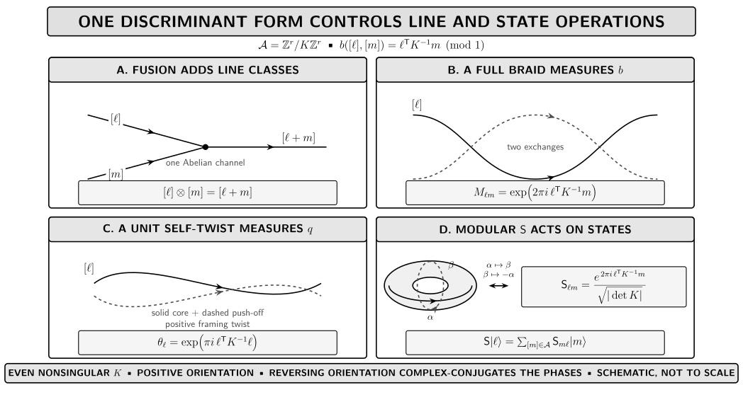
For an even nonsingular $K$, the discriminant group $\mathcal A=\mathbb Z^r/K\mathbb Z^r$ supplies the line labels and fusion, while $K^{-1}$ supplies their nondegenerate bilinear pairing. The positive full braid gives $M_{\ell m}$, a positive unit framing twist gives $\theta_\ell$, and the normalized pairing gives the orientation-preserving torus modular map $(\alpha,\beta)\mapsto(\beta,-\alpha)$. Reversing the orientation complex-conjugates the phases. The diagram is schematic, not to scale, and does not extend the bosonic quadratic formula to odd $K$ or assert a non-Abelian modular-category classification.

The one-component theory fixes the normalization

For $K=(k)$ with $k\ne0$, the action is

$$S_k[a] = \frac{k}{4\pi} \int_M a\wedge da.$$

The bosonic oriented theory has even $k$. Its lines are $n\in\mathbb Z_{\lvert k\rvert}$ and

$$\begin{aligned} [n]\otimes[m] &=[n+m], \\ M_{nm} &=\exp\left(\frac{2\pi i\,nm}{k}\right), \\ \theta_n &=\exp\left(\frac{\pi i\,n^2}{k}\right). \end{aligned}$$

The sign of $k$ records chirality: $k\mapsto-k$ complex-conjugates the braiding and spins. The smallest nontrivial bosonic control is $k=2$. It has two lines, $0$ and $1$, with

$$1\otimes1=0, \qquad M_{11}=-1, \qquad \theta_1=i.$$

Thus the nontrivial line is a semion. The $k=-2$ theory contains the anti-semion with $\theta_1=-i$.

The tempting $k=1$ substitution illustrates the spin caveat. After quotienting by all local particles, $\mathbb Z/K\mathbb Z$ is trivial and every fixed-spin state-space block is one-dimensional. If the local fermion is instead retained as a transparent line, the labels are $\mu\in\mathbb Z_{2\lvert k\rvert}$ for odd $k$, and $\mu$ and $\mu+k$ differ by fusion with that fermion. Thus $U(1)_1$ has the identity and a transparent fermion in the retained-line convention even though its fixed-spin block has one state. In either convention the theory is not a trivial oriented bosonic theory: odd $k$ needs spin structure and retains an invertible framing response. See Okuda, Saito, and Yokoyama 2021, § 4.1, printed p. 13, arXiv v2 PDF. Conversely, $k=0$ is not a finite Chern–Simons TQFT at all; its kinetic form is degenerate.

Canonical quantization gives the finite state count

Put the theory on $\mathbb R\times\Sigma_g$ and choose temporal gauge. Flat compact connections are characterized by their holonomies around the $2g$ cycles of a symplectic basis $\{\alpha_i,\beta_i\}_{i=1}^g$. On one handle, exponentiated holonomies obey a finite Heisenberg relation whose central phase is the same bilinear pairing $b$ that appears in braiding:

$$U_\ell V_m = \exp\left( 2\pi i\,\ell^{\mathsf T}K^{-1}m \right) V_m U_\ell.$$

The irreducible representation associated with one handle has dimension $\lvert\mathcal A\rvert=\lvert\det K\rvert$. Independent handles tensor, so

$$\boxed{ \dim\mathcal H(\Sigma_g) = \lvert\det K\rvert^g }.$$

For a teaching derivation of the compact torus Heisenberg algebra and its multi-component $K$-matrix extension, see Tong 2016, §§ 5.2.3–5.2.4, printed pp. 161–166, especially eqs. (5.27)–(5.28) and (5.31)–(5.32), arXiv v2 PDF. Those lectures use the quantum Hall effective-theory setting; the global compact and spin qualifications on this page still come from the specialist sources.

Belov and Moore obtain this genus-$g$ count in Belov and Moore 2005, § 5.3, printed p. 26, prose after eq. (5.17), arXiv v1 PDF. In the bosonic even-$K$ theory, a torus basis may be indexed by $[\ell]\in\mathcal A$, and the orientation-preserving modular generator $(\alpha,\beta)\mapsto(\beta,-\alpha)$ has matrix

$$\mathsf S_{\ell m} = \frac{1}{\sqrt{\lvert\det K\rvert}} \exp\left( 2\pi i\,\ell^{\mathsf T}K^{-1}m \right)$$

in the chosen positive convention. Orientation reversal conjugates it. Finite Fourier orthogonality gives

$$(\mathsf S^2)_{\ell n} = \delta_{[\ell],[-n]},$$

so two applications give charge conjugation rather than the identity. This is the algebraic check that $\mathsf S$ represents the signed, orientation-preserving cycle map, not a bare orientation-reversing swap. Spin theories instead have spin-structure-resolved blocks; the unqualified bosonic matrix must not be copied into an odd-$K$ theory. See Belov and Moore 2005, § 5.6.1, printed p. 35, eqs. (5.45)–(5.46), arXiv v1 PDF.

Closing the time direction supplies the independent gluing check

$$Z(\Sigma_g\times S^1) = \operatorname{Tr}_{\mathcal H(\Sigma_g)}\mathbf 1 = \lvert\det K\rvert^g,$$

with the induced product tangential structure and the chosen framing understood. This displayed equality is in the ordinary bosonic vector-valued theory. In a spin TQFT, the spin structure along the time circle can select a trace or a graded/supertrace-type closure, so the formula must be refined rather than copied unchanged. State counting, braiding, and surgery therefore probe the same finite pairing from three different directions in the declared bosonic scope.

First application: the three-model topological thread

The compact Abelian thread compares three descriptions in $2+1$ dimensions. It does not infer their equivalence from a shared local equation or a matching state count.

For compact $BF_N$ with $N\in\mathbb Z_{>0}$, take

$$K_{\mathrm{BF}} = \begin{pmatrix} 0 & N\\ N & 0 \end{pmatrix}, \qquad K_{\mathrm{BF}}^{-1} = \begin{pmatrix} 0 & 1/N\\ 1/N & 0 \end{pmatrix}.$$

Writing the two connections as $(A,B)$ gives

$$\begin{aligned} S_{K_{\mathrm{BF}}} &= \frac{N}{4\pi} \int_M \left( A\wedge dB+B\wedge dA \right) \\ &= \frac{N}{2\pi}\int_M B\wedge dA - \frac{N}{4\pi}\int_{\partial M}A\wedge B. \end{aligned}$$

Thus the symmetric $K$-matrix action equals the usual compact $BF_N$ action on a closed manifold. With a boundary, the explicit last term changes the polarization and cannot be dropped without a boundary convention.

A line is labeled by an electric–magnetic pair $(e,m)\in\mathbb Z_N\oplus\mathbb Z_N$. The formulas above give

$$\begin{aligned} b\bigl((e,m),(e',m')\bigr) &= \frac{em'+me'}{N} \pmod1, \\ q(e,m) &= \frac{em}{N} \pmod1, \\ \dim\mathcal H_{\mathrm{BF}_N}(\Sigma_g) &= N^{2g}. \end{aligned}$$

Pure electric and pure magnetic lines have trivial self-spin, while taking one around the other produces $e^{2\pi i/N}$ for unit charges. This is the finite clock–shift algebra in the state-space language.

Untwisted finite $\mathbb Z_N$ gauge theory has the same bounded electric and magnetic line data and

$$\dim\mathcal H(\Sigma_g) = \lvert H^1(\Sigma_g;\mathbb Z_N)\rvert = N^{2g}.$$

The equality with compact $BF_N$ becomes a theory-level statement only after the global compact sectors, automorphism-weighted finite-bundle sum, normalization, bordism maps, and boundary data are matched. A fixed cocycle weight is an invertible response; summing bundles produces the dynamical Dijkgraaf–Witten theory. The finite-bundle sum and state-space construction are explicit in Dijkgraaf and Witten 1990, §§ 6.2–6.3, printed pp. 415–417, eqs. (6.8)–(6.17). The automorphism-weighted measure and exact gluing contraction are developed in Freed and Quinn 1993, § 2, arXiv v3 internal printed pp. 9–13, especially eq. (2.1) and Theorem 2.13 with eq. (2.17), PDF.

A bosonic cyclic twist $r\in\mathbb Z_N$ has a continuum presentation

$$K_{N,r} = \begin{pmatrix} 2r & N\\ N & 0 \end{pmatrix}, \qquad \lvert\det K_{N,r}\rvert=N^2.$$

The twist can change the Smith normal form, fusion group, braiding, and spins even though it leaves the genus-$g$ dimension $N^{2g}$ unchanged. Therefore equal state counts are a check, not a complete invariant. In the notation of Kapustin and Seiberg, the diagonal entry is $p\sim p+2N$: the ordinary oriented bosonic Dijkgraaf–Witten class is $p=2r$, while odd $p$ is a spin refinement. Kapustin and Seiberg give the compact $BF$ fields, integer level, and cyclic twist identification in Kapustin and Seiberg 2014, §§ 3 and 5, printed pp. 9–13 and 20–21, eqs. (3.1)–(3.16) and (5.1)–(5.3), arXiv v2 PDF.

The rows compare one bounded diagnostic package; matching entries do not by themselves prove that two globally defined theories are equivalent.

Dynamical model	Finite line labels	Positive mutual phase	Genus-g state count	Global qualification
Bosonic compact U(1), even level k	ℤ divided by kℤ	exp(2πi nm/k)	|k|g	Odd k is a separate spin theory with a refined line convention.
Compact BF level N	ℤN ⊕ ℤN	exp[2πi(em′ + me′)/N]	N2g	Both compact fields and all flux sectors are summed.
Untwisted finite ℤN gauge theory	Electric and magnetic labels	exp(2πi/N) for unit electric–magnetic linking	N2g	Bundles are summed with groupoid weights; a fixed bundle gives only a phase.

The forthcoming compact BF treatment will develop the higher-form equations, torsion sectors, and boundary polarizations. The forthcoming finite-gauge treatment will develop the bundle groupoid, cocycle twists, and gluing measure. The present page owns only the K-matrix computation and the bounded comparison.

Spin refinements and other failure modes

For odd $K$, first declare what is meant by a line label. If all local particles, including the local fermion, are quotiented, the discriminant group

$$\mathcal D=\mathbb Z^r/K\mathbb Z^r$$

and bilinear pairing $b$ remain meaningful, and the fixed-spin state-space dimension remains $\lvert\det K\rvert^g$. The naive bosonic expression

$$\frac12\ell^{\mathsf T}K^{-1}\ell$$

does not descend to a function on $\mathcal D$: shifting $\ell\mapsto\ell+Kn$ may change it by a half-integer because a local particle may be fermionic. Topological spin is then defined only with the spin-dependent quadratic refinement, or equivalently only up to the sign of that local fermion in the quotient description.

If the transparent local fermion is retained, the line set is enlarged. In one-component odd-level $U(1)_k$, it is $\mathbb Z_{2\lvert k\rvert}$; the line $W_k$ is transparent and has $\theta=-1$, while the spin-structure-resolved state-space blocks still have $\lvert k\rvert^g$ states. In the same positive convention,

$$M_{\mu\nu} = \exp\left( \frac{2\pi i\,\mu\nu}{k} \right), \qquad \theta_\mu = \exp\left( \frac{\pi i\,\mu^2}{k} \right), \qquad \mu,\nu\in\mathbb Z_{2\lvert k\rvert}.$$

For $f=[k]$, these equations give $M_{f\nu}=1$ and $\theta_f=(-1)^k=-1$. The two line conventions are therefore not contradictory counts.

Belov and Moore encode the discriminant spin data as $(\mathcal D,b,[q])$. A characteristic vector constructs a representative of $q$; it is not an extra freely selectable phase label. The full quantum spin Chern–Simons invariant also records the lattice signature modulo $24$ once the framing convention is fixed. See Belov and Moore 2005, § 1, printed pp. 4–5, eqs. (1.4)–(1.7), and § 5.6, printed pp. 32–36, arXiv v1 PDF. The retained-fermion one-component description is explicit in Okuda, Saito, and Yokoyama 2021, § 4.1, printed p. 13, arXiv v2 PDF.

Several other ceilings matter:

• A boundary makes the theory relative. The bulk variation leaves a boundary term. A polarization, boundary condition, counterterm, or edge theory is additional data; the bulk $K$ matrix does not choose one.
• A framing phase survives finite line triviality. A unimodular $K$ has no nontrivial discriminant-group lines, but its signature can still carry an invertible gravitational/framing response.
• The global charge lattice is physical input. Changing the compact gauge group, allowed monopoles, or local matter can change which Wilson charges are identified even if the local differential form looks the same.
• A degenerate matrix is a different problem. If $\det K=0$, the inverse, finite line pairing, and $\lvert\det K\rvert^g$ count do not exist.
• Finite Abelian data are not a category theorem. Associator phases and their coherence are additional even when every fusion channel is one-dimensional. Fusion multiplicities, non-Abelian braid matrices, and modular-category classification require still more structures and hypotheses.

What the K matrix does not determine

The finite package

$$(\mathcal A,b,q)$$

determines the bounded bosonic line fusion, monodromy, and spin used here. It does not, without further input, determine

• a microscopic Hamiltonian or a unique infrared realization;
• a preferred boundary condition or edge conformal field theory;
• the complete framing counterterm and absolute gravitational response;
• a canonical identification between two presentations with the same determinant;
• a non-Abelian extension or a theorem classifying modular tensor categories; or
• the electromagnetic charge vector, Hall response, and quasiparticle embedding used in a quantum Hall material.

This is why a $K$ matrix can give exact topological calculations without being a complete phase specification.

Check your understanding

1. Why does the bosonic spin descend to the quotient? Show directly that $q([\ell])=\tfrac12\ell^{\mathsf T}K^{-1}\ell$ is unchanged modulo one under $\ell\mapsto\ell+Kn$.

Solution

The change is

$$n^{\mathsf T}\ell+\frac12n^{\mathsf T}Kn.$$

The first term is integral. The second is integral precisely because an even integral lattice has $n^{\mathsf T}Kn\in2\mathbb Z$. For odd $K$ this argument can fail by one half, which is why spin refinement is extra data.

2. Compute the semion control. For $K=(2)$, find the line group, nontrivial line spin, mutual full braid of two nontrivial lines, and the genus-two state count.

Solution

The line group is $\mathbb Z_2$. For its generator,

$$\theta_1=e^{\pi i/2}=i, \qquad M_{11}=e^{\pi i}=-1.$$

The state count is

$$\dim\mathcal H(\Sigma_2)=2^2=4.$$

3. Separate a determinant check from a theory equivalence. Compare $K_{\mathrm{BF}}=\left(\begin{smallmatrix}0&N\\N&0\end{smallmatrix}\right)$ with untwisted finite $\mathbb Z_N$ gauge theory.

Solution

Both have $N^{2g}$ states on $\Sigma_g$ and the same unit electric–magnetic linking phase. These checks do not establish equivalence until the compact global sectors, finite-bundle measure, normalization, bordism maps, and boundary data are matched. Local flatness alone is insufficient.

4. Diagnose a failed use of the formula. What goes wrong for $K=\operatorname{diag}(2,0)$?

Solution

The determinant vanishes, so $K^{-1}$ does not exist and the quotient $\mathbb Z^2/K\mathbb Z^2$ has an infinite component. Continuous zero modes remain. Neither the finite braiding pairing nor the $\lvert\det K\rvert^g$ state count applies.

Continue to relative theories and physical realizations

The forthcoming Operators, Boundaries, and Relative Topological Theories will use these explicit line phases inside boundary, interface, and gluing problems. For material response, Fractional Quantum Hall Fluids and Abelian Topological Orders and K-Matrix Data will add the electromagnetic charge vector, filling fraction, quasiparticle charge, and microscopic interpretation. Theorem-level non-Abelian Chern–Simons theory and modular-category classification remain Mathematical QFT handoffs rather than claims of this finite Abelian calculation.

References

• Belov, Dmitriy M., and Gregory W. Moore. “Classification of Abelian Spin Chern–Simons Theories.” arXiv:hep-th/0505235v1 (2005). arXiv record.
• Dijkgraaf, Robbert, and Edward Witten. “Topological Gauge Theories and Group Cohomology.” Communications in Mathematical Physics 129, no. 2 (1990): 393–429. DOI 10.1007/BF02096988.
• Freed, Daniel S., and Frank Quinn. “Chern–Simons Theory with Finite Gauge Group.” Communications in Mathematical Physics 156, no. 3 (1993): 435–472. DOI 10.1007/BF02096860. Open PDF, arXiv:hep-th/9111004v3; v1 and v2 were withdrawn.
• Kapustin, Anton, and Natalia Saulina. “Topological Boundary Conditions in Abelian Chern–Simons Theory.” Nuclear Physics B 845 (2011): 393–435. DOI 10.1016/j.nuclphysb.2010.12.017. Open PDF, arXiv:1008.0654v2.
• Kapustin, Anton, and Nathan Seiberg. “Coupling a QFT to a TQFT and Duality.” Journal of High Energy Physics 2014, no. 4 (2014): 001. DOI 10.1007/JHEP04(2014)001. Open PDF, arXiv:1401.0740v2.
• Okuda, Takuya, Koichi Saito, and Shuichi Yokoyama. “U(1) Spin Chern–Simons Theory and Arf Invariants in Two Dimensions.” Nuclear Physics B 962 (2021): 115272. DOI 10.1016/j.nuclphysb.2020.115272. Open PDF, arXiv:2005.03203v2.
• Tong, David. “Lectures on the Quantum Hall Effect.” arXiv:1606.06687v2 (2016). DOI 10.48550/arXiv.1606.06687. Open PDF, arXiv:1606.06687v2.
• Witten, Edward. “Quantum Field Theory and the Jones Polynomial.” Communications in Mathematical Physics 121, no. 3 (1989): 351–399. DOI 10.1007/BF01217730. Open PDF.