Symmetry TFT: Encoding Symmetry, Anomaly, and Gauging

A symmetry topological field theory packages part of the symmetry data of a $d$-dimensional quantum field theory into a topological theory in $d+1$ dimensions. In the controlled sandwich construction used here, the one-higher-dimensional bulk is placed between a topological symmetry boundary and a generally non-topological physical boundary. Bulk topological operators then encode symmetry defects, their linking or fusion data, and possible anomalies; the symmetry boundary selects an absolute realization such as a global form or gauging choice; the physical boundary contains the actual QFT dynamics.

This is a powerful separation of symmetry from dynamics, not a universal reconstruction theorem. The page works with explicitly constructed finite, discrete, Abelian, or otherwise topological sectors for which the bulk and both boundary roles are known. It does not assume that every relative QFT has a symmetry-TFT realization, that every gauging is a change of boundary condition, or that the auxiliary bulk determines a boundary Hamiltonian.

Required background. Operators, Boundaries, and Relative Topological Theories supplies the vector- or covector-valued boundary assignment and the distinction between a physical boundary and a sewing cut. Anomaly Polynomials and Inflow supplies the orientation convention for inverse bulk and boundary variations. Higher-Group Operators, Gauging, and Anomalies supplies the rule that gaugeability belongs to the full background-coupled family, not to an isolated current. Helpful background. Non-Invertible Anomalies and RG Constraints sets limits on obstruction arguments, while Background Responses and Invertible Phases separates a fixed-background phase from a dynamical topological sum.

A symmetry TFT is a sandwich, not the boundary theory

Let $\mathcal S$ denote a specified symmetry datum and let $Z(\mathcal S)$ be a topological theory in $d+1$ dimensions. Suppose that $Z(\mathcal S)$ admits

• a topological boundary condition $B_{\mathrm{sym}}^{\mathcal S}$ that realizes the chosen absolute form of the symmetry, and
• a physical boundary condition $B_{\mathrm{phys}}^{\mathcal T,\sigma}$ that contains a $d$-dimensional QFT $\mathcal T$ and its coupling $\sigma$ to the symmetry data.

Compactifying the interval between them gives the bounded sandwich

$$\mathcal T_\sigma = \operatorname{Comp}_I \left( B_{\mathrm{sym}}^{\mathcal S} \ \middle|\ Z(\mathcal S) \ \middle|\ B_{\mathrm{phys}}^{\mathcal T,\sigma} \right).$$

The vertical bars mean adjoining boundaries of the same bulk, not tensor factors. The symmetry boundary is topological so that it can be moved without probing local length scales. The physical boundary need not be topological: it may carry propagating fields, an RG flow, a stress tensor, and nontrivial correlation functions.

On a spatial $d$-manifold $X$, the same structure can be read as a pairing in the bulk state space,

$$Z_{\mathcal T_\sigma}(X) = \left\langle B_{\mathrm{sym}}^{\mathcal S} \middle| B_{\mathrm{phys}}^{\mathcal T,\sigma} \right\rangle_{\mathcal H_{Z(\mathcal S)}(X)}.$$

This formula is schematic until the field space, tangential structure, boundary conditions, and normalization of the pairing have been supplied. When the bulk is invertible, the relevant state space is a line and the formula reduces to anomaly-line inflow. A symmetry TFT can instead be noninvertible and have a higher-dimensional state space, as finite gauge and compact $BF$ theories do.

The controlled sandwich and the distinction between topological and physical boundaries are developed in Bhardwaj and Schäfer-Nameki 2025, Introduction and §§ 2.4, 2.6–2.7, arXiv v3, especially Statement 2.1 and eqs. (2.40), (2.68)–(2.72), PDF. Their detailed constructions concern declared finite or categorical settings; the sandwich is not asserted here as an existence theorem for arbitrary QFTs.

The next figure records exactly which passages are automatic. In particular, look at the dashed arrows: neither extension to lower codimension nor a symmetry-TFT realization follows from ordinary or relative data alone.

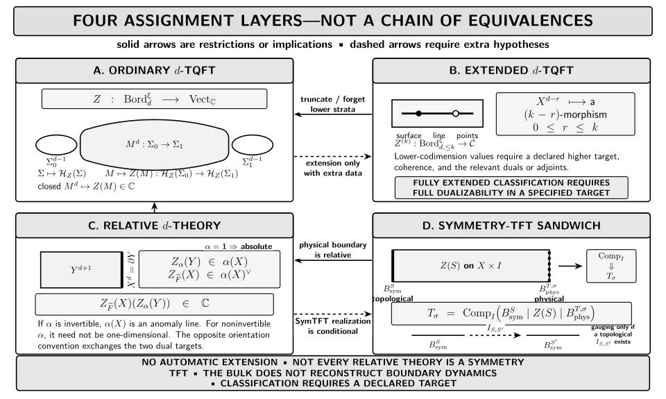
Ordinary, extended, relative, and symmetry-TFT data are related by restrictions and conditional constructions, not by four equivalences. Extension adds lower-codimension assignments in a declared higher target. A relative $d$-theory supplies compatible boundary data relative to an extended $(d+1)$-theory; for an invertible bulk its boundary value pairs with a bulk state in a one-dimensional anomaly line. In the bounded symmetry-TFT sandwich, a suitable topological symmetry boundary and a physical boundary compactified across an interval recover the $d$-dimensional theory. Gauging or condensation changes the symmetry boundary only when the required topological interface exists. The diagram is schematic and does not assert universal symmetry-TFT existence, reconstruct boundary dynamics, or prove a dualizability or classification theorem.

Bulk operators separate symmetry from dynamics

A topological operator in $Z(\mathcal S)$ can be brought to either boundary. At the symmetry boundary it is projected, condensed, or allowed to end according to $B_{\mathrm{sym}}^{\mathcal S}$. At the physical boundary it becomes a symmetry defect or an endpoint for a charged operator of $\mathcal T$. Linking and fusion in the bulk therefore constrain the composition and transport of boundary symmetry defects without specifying their local dynamical realization.

This division immediately gives a non-reconstruction test. Let $\mathcal N$ be a neutral, anomaly-free QFT on which $\mathcal S$ acts trivially. Replacing

$$\mathcal T \longmapsto \mathcal T\otimes\mathcal N$$

does not change the symmetry action, its topological defect algebra, or its anomaly. It can nevertheless change the stress tensor, local spectrum, correlation functions, scales, and RG behavior. The same $Z(\mathcal S)$ and symmetry boundary can therefore support inequivalent physical boundaries.

Conversely, changing the symmetry boundary while holding the physical boundary fixed can change which bulk operators become genuine boundary defects and which remain attached to higher-dimensional surfaces. That operation changes the absolute realization of the symmetry without pretending to derive the boundary dynamics.

Gauging is a boundary change only when an interface exists

Suppose two topological symmetry boundaries are connected by a topological interface

$$\mathcal I_{\mathcal S,\mathcal S'}: B_{\mathrm{sym}}^{\mathcal S} \longrightarrow B_{\mathrm{sym}}^{\mathcal S'}.$$

If the physical boundary is left fixed, inserting the interface and compressing the interval can implement a controlled gauging, condensation, orbifold, or change of global form:

$$\operatorname{Comp}_I \left( B_{\mathrm{sym}}^{\mathcal S} \middle| Z \middle| B_{\mathrm{phys}} \right) \longrightarrow \operatorname{Comp}_I \left( B_{\mathrm{sym}}^{\mathcal S'} \middle| Z \middle| B_{\mathrm{phys}} \right).$$

Three hypotheses matter.

First, the required topological interface must actually exist. An anomaly can obstruct it, and a proposed condensate may fail isotropy, maximality, or boundary compatibility. Second, the operation must preserve the field and tangential structures used to define the bulk. Third, the physical boundary is held fixed; changing it at the same time would mix a symmetry operation with a change of the QFT.

There is also an important continuous-symmetry ceiling. Gauging a finite subgroup or a flat $U(1)$ background can often be represented by a topological boundary manipulation. Ordinary dynamical gauging of a continuous $U(1)$ introduces a propagating photon and generally changes the symmetry TFT itself, rather than merely changing a boundary of the old one. Antinucci and Benini make this distinction explicit in Antinucci and Benini 2025, §§ II and IV, arXiv v4, printed pp. 2–4 and 7–9, PDF.

Five-dimensional BF encodes electric and magnetic one-form data

The reciprocal four-dimensional application is a five-dimensional Abelian $BF$ theory. Let $X_5$ be a closed oriented manifold for the global definition, and later allow the boundary $Y_4=\partial X_5$. Take compact $U(1)$ two-form gauge fields $B_e$ and $B_m$ and the Lorentzian weight $e^{iS_5}$ with

$$S_5 = \frac{N}{2\pi} \int_{X_5} B_e\wedge dB_m, \qquad N\in\mathbb Z_{>0}.$$

The displayed form integral is local notation. Intrinsically, $B_e$ and $B_m$ are compact higher connections, their three-form curvatures have $2\pi$-integral periods, and the exponentiated action is defined by a differential-cohomology or cocycle pairing. Integer $N$ is required by large gauge invariance. Integrating out one field makes the other locally flat but leaves finite $\mathbb Z_N$ holonomy sectors; flat does not mean globally zero. The compact global construction is reviewed in Gaiotto, Kapustin, Seiberg, and Willett 2015, § 6, arXiv v2, printed pp. 33–38, especially eqs. (6.8)–(6.13), PDF.

For disjoint closed oriented surfaces $\Gamma,\Gamma'\subset X_5$ whose homology classes admit the ordinary integer linking construction, define

$$U_e(\Gamma) = \exp\!\left(i e\int_\Gamma B_e\right), \qquad U_m(\Gamma') = \exp\!\left(i m\int_{\Gamma'}B_m\right), \qquad e,m\in\mathbb Z_N.$$

For example, if both supports lie in $S^5$, $\mathbb R^5$, or a local homology ball and $\Gamma=\partial C_3$, set $\operatorname{Lk}(\Gamma,\Gamma')=C_3\mathbin{\cdot}\Gamma'$. With the positive linking convention inherited from compact $BF$ theory,

$$U_e(\Gamma)\,U_m(\Gamma') = \exp\!\left( \frac{2\pi i\,em}{N} \operatorname{Lk}(\Gamma,\Gamma') \right) U_m(\Gamma')\,U_e(\Gamma).$$

Reversing the orientation of either support, or reversing the operator-order convention, complex-conjugates the phase. The $N$th powers are trivial. Thus the electric and magnetic surface families form a finite Heisenberg pair rather than two independent commuting label sets. On a general manifold where neither support bounds, the corresponding torsion or differential-cohomology pairing replaces this integer linking number.

Canonical quantization on a closed oriented four-manifold $M_4$ turns intersection into equal-time commutation. In a torsion-free example,

$$\dim\mathcal H_{BF}(M_4) = N^{b_2(M_4)}.$$

In particular,

$$\dim\mathcal H_{BF}(T^4)=N^6.$$

There is one $N$-valued coordinate for each generator of $H^2(M_4;\mathbb Z)$; the conjugate magnetic flux acts by finite translation rather than providing a second independent label. With torsion, the compact cochain or differential-cohomology pairing and the gauge-volume normalization must be retained; under the same polarization used on the compact-$BF$ page, the finite state set is governed by $H^2(M_4;\mathbb Z_N)$.

Duan, Jia, and Lee derive the level-$N$ five-dimensional action, its canonical quantization, the surface-operator algebra, and the torsion-free state count in Duan, Jia, and Lee 2025, § 2, arXiv v3, printed pp. 8–22, especially eqs. (2.1), (2.11)–(2.18), PDF.

Boundary polarization exposes the mixed anomaly

Opening $X_5$ gives

$$\begin{aligned} \delta S_5 = \frac{N}{2\pi} \biggl[ &\int_{X_5} \left( \delta B_e\wedge dB_m - \delta B_m\wedge dB_e \right) \\ &+ \int_{Y_4} B_e\wedge\delta B_m \biggr]. \end{aligned}$$

The bulk equations are $dB_e=dB_m=0$. The boundary term supplies the presymplectic pairing

$$\Omega_{Y_4} = \frac{N}{2\pi} \int_{Y_4} \delta B_e\wedge\delta B_m,$$

up to the overall field-space sign convention. A topological boundary must choose a maximal commuting, or maximal isotropic, half of this data. The displayed representative is directly well posed with $B_m$ fixed, since then $\delta B_m|_{Y_4}=0$. To make a general fixed-$B_e$ polarization well posed, add

$$S_{\mathrm{ct}} =-\frac{N}{2\pi} \int_{Y_4} B_e\wedge B_m.$$

The new boundary potential is $-\frac{N}{2\pi}\int_{Y_4}\delta B_e\wedge B_m$, so fixing $B_e$ now annihilates it. Homogeneous $B_e|_{Y_4}=0$ is the special case that already kills the original boundary term. Attempting to impose arbitrary values for both conjugate fields is not a polarization.

The same obstruction appears under a background gauge transformation. For $B_e\mapsto B_e+d\Lambda_e$,

$$\Delta_{\Lambda_e}S_5 = \frac{N}{2\pi} \int_{Y_4} \Lambda_e\wedge dB_m.$$

The asymmetric representative is invariant under $B_m\mapsto B_m+d\Lambda_m$. With the exact counterterm above,

$$\Delta_{\Lambda_e}(S_5+S_{\mathrm{ct}})=0, \qquad \Delta_{\Lambda_m}(S_5+S_{\mathrm{ct}}) =-\frac{N}{2\pi} \int_{Y_4} \Lambda_m\wedge dB_e.$$

The counterterm transfers the displayed variation between the two background symmetries, but it cannot make the mutual anomaly class vanish. The physical boundary must transform by the inverse phase.

For a four-dimensional gauge-theory boundary, the two bulk surface families encode electric and magnetic one-form data. In the elementary global-form choices, one polarization gives the $SU(N)$-type theory in which Wilson lines are genuine and magnetic lines are surface-attached; the complementary polarization gives the $PSU(N)$-type choice with the roles exchanged. Composite $N$, discrete theta angles, and non-spin manifolds can require additional maximal-isotropic subgroups and quadratic refinements, so the two coordinate choices are not a complete classification.

A fully discrete mixed-anomaly control is the $k=0$ global form

$$\bigl(SU(4)/\mathbb Z_2\bigr)_0,$$

one of the two discrete-theta variants commonly denoted $SO(6)$ Yang–Mills. It is the $N=4$, $P=Q=2$, $k=0$ case in the partial-gauging construction. The $k=1$ case instead has a $\mathbb Z_4$ one-form symmetry and must not be identified with the example below.

Let $a_e,b_e,a_m,b_m$ be dynamical degree-two $\mathbb Z_2$ cochains on a triangulated oriented five-manifold. A finite cochain symmetry-TFT action weight is

$$W_{\mathrm{cochain}}(X_5) = \exp\!\left[ \pi i \int_{X_5} \left( a_e\smile\delta b_e + a_m\smile\delta b_m + a_m\smile\operatorname{Bock}(a_e) \right) \right].$$

The full finite partition function sums this weight over the gauge groupoid with its normalization; the displayed factor is the part needed for the field equation and anomaly test.

For fixed background cocycles $A_e,A_m$, the corresponding anomaly inflow is

$$\exp\!\left( \pi i \int_{X_5} A_m\smile\operatorname{Bock}(A_e) \right).$$

The Bockstein comes from $0\to\mathbb Z_2\to\mathbb Z_4\to\mathbb Z_2\to0$. Varying $a_m$ gives the cochain equation

$$\delta b_m=\operatorname{Bock}(a_e).$$

Consequently a Dirichlet condition on $b_m$ forces the compatible Dirichlet condition on $a_e$, whereas gauging the electric factor requires the complementary, summed boundary condition on $a_e$. The two gauging boundary conditions therefore cannot be imposed together unless extra boundary or inflow data cancel the class. This is the promised boundary-condition derivation of the mixed anomaly, not merely a noncommuting-operator slogan.

The exact cochain model and boundary obstruction appear in Bhardwaj et al. 2024, § 4.5, arXiv v2, printed p. 113, especially eqs. (4.265)–(4.267), PDF. Duan, Jia, and Lee relate the same $N=4$, $P=Q=2$, $k=0$ example to compact five-dimensional $BF$ and partial gauging in Duan, Jia, and Lee 2025, §§ 2.3–2.4 and 4.3, arXiv v3, printed pp. 18–23 and 54–56, PDF.

There is a related continuous control, but it is a different global theory. In the unit electric–magnetic charge-lattice normalization, four-dimensional Maxwell theory has $U(1)^{(1)}_e$ and $U(1)^{(1)}_m$ backgrounds with anomaly polynomial

$$I_6 = \frac{dB_e}{2\pi} \wedge \frac{dB_m}{2\pi}.$$

The corresponding five-dimensional representative is

$$S_{5,\mathrm{inflow}} = \frac{1}{2\pi} \int_{X_5} B_e\wedge dB_m.$$

In this use the fields are fixed backgrounds, so the functional is an invertible anomaly response. Summing compact $B_e,B_m$ instead gives the noninvertible finite $BF_N$ symmetry TFT above. Setting $N=1$ in the latter produces a trivial finite topological Hilbert space; it does not reproduce the continuous Maxwell symmetry TFT. The symmetry data also do not determine the Maxwell coupling or charge normalization. This statement concerns pure compact Maxwell theory; charged matter can explicitly break one or both one-form symmetries. The Maxwell mixed anomaly and simultaneous-gauging obstruction are derived in Gaiotto, Kapustin, Seiberg, and Willett 2015, § 4.1, arXiv v2, printed pp. 14–16, especially eqs. (4.1)–(4.3), PDF.

First application: the same sandwich test across three models

The Abelian Chern–Simons, compact $BF$, and finite-gauge rows below share a boundary-and-gauging diagnostic. They are not equivalent theories, and their operators live in different dimensions.

One symmetry-boundary diagnostic across the three-model topological thread

Auxiliary topological bulk	Bulk symmetry datum	Topological symmetry boundary	Controlled gauging change	What remains in the physical boundary
Bosonic Abelian Chern–Simons	Discriminant lines with fusion, full braid, spin, and framing data	A compatible Lagrangian condensate, together with the chiral obstruction test	A topological condensation interface changes the allowed genuine line set when it exists	Edge dynamics, local operator spectrum, velocity, couplings, and the choice of physical boundary theory
Compact BF	Complementary electric and magnetic operators with a finite Heisenberg pairing	A maximal-isotropic polarization selecting which operators may end or remain genuine	Exchange or partial gauging through an admissible polarization-changing interface	The gauge-theory dynamics, matter screening, RG flow, and any propagating boundary fields
Finite Dijkgraaf–Witten	Finite bundles, cocycle weight, and transgressed flux–charge defect data	A subgroup map with a cochain trivializing the restricted cocycle in the elementary class	A finite groupoid sum or orbifold only when the restricted anomaly is trivialized	Which boundary QFT realizes the symmetry, its local observables, and its phase dynamics

The comparison isolates the common mechanism:

$$\text{bulk topological data} \;+\; \text{symmetry boundary} \;+\; \text{physical boundary}.$$

In Abelian Chern–Simons theory the topological operators are lines and an ordinary bosonic vacuum boundary is tested by a Lagrangian subgroup together with vanishing chiral obstruction. The discriminant lines, their linking data, and the controlled Abelian boundary condition are developed in Kapustin and Saulina 2011, §§ 2–4, arXiv v2, printed pp. 2–16, PDF. In compact $BF$ theory, complementary Wilson supports form a finite Heisenberg pair and a boundary chooses a polarization. In finite Dijkgraaf–Witten theory, the bulk sum is over finite bundles with inverse-automorphism measure and a cocycle twist; an elementary subgroup boundary $H\to G$ additionally needs a cochain $\vartheta$ with

$$\delta\vartheta=\omega|_H.$$

If the restricted class is nonzero, that elementary gauging boundary does not exist. This formula uses the boundary-orientation convention declared here; reversing the boundary orientation inverts the cocycle. The elementary subgroup-and-cochain boundary condition is developed in Fuchs, Schweigert, and Valentino 2014, §§ 2.5 and 3.2, arXiv v3, internal printed pp. 12–13 and 17–18, especially eq. (3.13), PDF. Dijkgraaf and Witten derive the finite-bundle sum, state spaces, and lattice cocycle factors in Dijkgraaf and Witten 1990, §§ 6.2–6.5, printed pp. 415–421, especially eqs. (6.8)–(6.27), PDF.

The rows therefore compare how a one-higher-dimensional topological system organizes symmetry and boundary choices. Equality of a line count, a Hilbert space dimension, or one linking phase would not prove equivalence of their bulk theories or boundary QFTs.

What the symmetry TFT does not determine

The sandwich can determine or constrain:

• topological symmetry defects and their fusion, linking, or braiding data;
• anomaly inflow and the incompatibility of certain boundary conditions;
• global-form and polarization choices;
• candidate finite gauging, condensation, or orbifold interfaces; and
• relative partition functions and topological protected quantities.

It does not, without additional input, determine:

• a local boundary Lagrangian, Hamiltonian, or stress tensor;
• scaling dimensions, OPE coefficients, ordinary correlation functions, or a mass spectrum;
• whether a boundary flows to a gapped, gapless, symmetry-breaking, or topologically ordered phase;
• a unique presentation of the topological bulk; or
• a universal categorical classification of continuous, noninvertible, nonsemisimple, or fully extended symmetries.

The neutral-spectator test already proves the first three non-implications. The remaining statements reflect extra choices of presentation, boundary data, and higher coherence. Even within Abelian models, matter can screen a putative center symmetry, torsion can invalidate a de Rham-only calculation, and a non-spin manifold can require quadratic refinements invisible in the naive form action.

Current work extends symmetry-TFT methods well beyond the finite examples, but the hypotheses and equivalence notions are still framework-dependent. A current analysis of three-dimensional finite non-Abelian symmetry TFTs also shows why one simple Dijkgraaf–Witten presentation need not be unique and can hide magnetic or boundary-attached operator data. Bergman, Heckman, Hübner, Migliorati, Yu, and Zhang 2026, abstract and § 1, current arXiv v2, printed pp. 1–7, PDF is used here only as a scope qualification, not as authority for the Abelian formulas above. Sources and current-version records for the research-sensitive claims on this page were checked through 2026-08-10.

Check your understanding

1. Count the five-dimensional BF states on a four-torus

For torsion-free $M_4=T^4$, verify $\dim\mathcal H_{BF}(T^4)=N^6$.

Solution

The second Betti number of the four-torus is

$$b_2(T^4)=\binom42=6.$$

In the $B_e$ polarization, each independent two-cycle carries one $\mathbb Z_N$ holonomy, while the $B_m$ holonomy is its conjugate shift operator rather than a second state label. Hence

$$\dim\mathcal H_{BF}(T^4)=N^{b_2(T^4)}=N^6.$$

2. Move the mixed-anomaly representative

Show that adding a boundary term proportional to $\int_{Y_4}B_e\wedge B_m$ can move the displayed gauge variation from the $B_e$ transformation to the $B_m$ transformation, but cannot make both variations disappear.

Solution

The bulk representative

$$\frac{N}{2\pi}\int_{X_5}B_e\wedge dB_m$$

varies by $\frac{N}{2\pi}\int_{Y_4}\Lambda_e\wedge dB_m$ under $B_e\mapsto B_e+d\Lambda_e$. The boundary term changes by contributions under both $B_e$ and $B_m$ transformations. Choosing its sign cancels the first displayed variation, but integration by parts leaves the reciprocal $B_m$ variation. The counterterm changes the anomaly representative; the nontrivial mixed class remains.

3. Test whether a manipulation is only a boundary change

Classify each operation:

1. gauge an anomaly-free finite subgroup through a known topological interface while keeping the physical boundary fixed;
2. dynamically gauge a continuous $U(1)$ and introduce a Maxwell photon;
3. tensor the physical boundary with a neutral QFT.

Solution

The first is the controlled boundary-change operation in the fixed symmetry TFT. The second changes the propagating content and generally requires a different symmetry TFT. The third changes only the physical boundary; it leaves the symmetry bulk and symmetry boundary unchanged while altering local dynamics. These three operations cannot be identified.

4. Find the failed polarization

Why can the electric and magnetic surface holonomies not both be treated as independent coordinates in the five-dimensional compact $BF_N$ Hilbert space?

Solution

Their operators obey the finite Heisenberg relation. When the supporting cycles intersect once,

$$U_eU_m=e^{2\pi i/N}U_mU_e.$$

Two operators with this commutator cannot be simultaneously diagonalized. Choosing the electric holonomies as coordinates makes the magnetic operators finite translations, and the converse choice exchanges their roles. Counting both as independent labels would square the state count and violate the canonical pairing.

Continue to theorem-level and holographic realizations

Symmetry TFTs, Anomaly Inflow, and Boundary Realizations will formulate the extended and categorical targets, boundary morphisms, duality hypotheses, and equivalence notions needed for theorem-level statements.

Boundary Global Symmetry, Bulk Gauge Symmetry, and Global Form will study how related distinctions appear in holographic bulk–boundary systems. Neither continuation is a prerequisite for the bounded models computed here.

References

• Antinucci, Andrea, and Francesco Benini. “Anomalies and Gauging of $U(1)$ Symmetries.” Physical Review B 111 (2025): 024110. DOI. Open PDF, current arXiv:2401.10165v4.
• Bergman, Oren, Jonathan J. Heckman, Max Hübner, Daniele Migliorati, Xingyang Yu, and Hao Y. Zhang. “On the SymTFTs of Finite Non-Abelian Symmetries.” arXiv:2603.12323v2 [hep-th] (2026). Stable record. Open PDF, current v2.
• Bhardwaj, Lakshya, Lea E. Bottini, Ludovic Fraser-Taliente, Liam Gladden, Dewi S. W. Gould, Arthur Platschorre, and Hannah Tillim. “Lectures on Generalized Symmetries.” Physics Reports 1051 (2024): 1–87. DOI. Open PDF, current arXiv:2307.07547v2.
• Bhardwaj, Lakshya, and Sakura Schäfer-Nameki. “Generalized Charges, Part II: Non-Invertible Symmetries and the Symmetry TFT.” SciPost Physics 19 (2025): 098. DOI. Open PDF, current arXiv:2305.17159v3.
• Dijkgraaf, Robbert, and Edward Witten. “Topological Gauge Theories and Group Cohomology.” Communications in Mathematical Physics 129, no. 2 (1990): 393–429. DOI. Open PDF.
• Duan, Zhihao, Qiang Jia, and Sungjay Lee. “Web of 4D Dualities, Supersymmetric Partition Functions and SymTFT.” Journal of High Energy Physics 2025, no. 1 (2025): 161. DOI. Open PDF, current arXiv:2410.10036v3.
• Fuchs, Jürgen, Christoph Schweigert, and Alessandro Valentino. “A Geometric Approach to Boundaries and Surface Defects in Dijkgraaf–Witten Theories.” Communications in Mathematical Physics 332, no. 3 (2014): 981–1015. DOI. Open PDF, current arXiv:1307.3632v3.
• Gaiotto, Davide, Anton Kapustin, Nathan Seiberg, and Brian Willett. “Generalized Global Symmetries.” Journal of High Energy Physics 2015, no. 2 (2015): 172. DOI. Open PDF, current arXiv:1412.5148v2.
• Kapustin, Anton, and Natalia Saulina. “Topological Boundary Conditions in Abelian Chern–Simons Theory.” Nuclear Physics B 845 (2011): 393–435. DOI. Open PDF, current arXiv:1008.0654v2.