Higher-Group Operators, Gauging, and Anomalies

Once a finite internal 2-group $(G,\mathcal A,\rho,[\beta])$ is fixed, its four main consequences follow in order. First, zero-form walls must transport one-form surfaces and their charged-line sectors, while a wall associator carries the surface labelled by $\beta$. Second, gauging must sum the complete constrained background family, or a closed anomaly-free subfamily, rather than treating the two factors as automatically independent. Third, the Postnikov class is symmetry structure, whereas an anomaly is a counterterm-invariant phase under the full coupled transformation. Fourth, only exact symmetry and anomaly data whose background families are identified across scales obey an RG matching statement.

This page treats finite internal 2-groups and a four-dimensional compact Abelian model with a finite electric surface network. Continuous differential forms supply a local orientation where useful, but they do not classify torsion, large-gauge, spin, or boundary data. The discussion assumes genuine operators in the declared global form and separates a necessary label or incidence check from the existence, normalization, and coherence of junction spaces.

Required background. Higher-Group Symmetry and Coupled Backgrounds supplies $(G,\mathcal A,\rho,[\beta])$, the coupled background constraint, and the wall–surface–line dictionary. Gauging a Higher-Form Symmetry supplies gaugeability, the finite groupoid sum, and the distinction between projection, attachment, and screening; its operator section fixes the attachment convention. What Is an Anomaly? supplies the obstruction test, while its local-versus-global comparison supplies counterterm equivalence and the local/global distinction.

Evidence scope, checked 9 August 2026. The operator, gauging, anomaly, RG, and compact-model claims below were checked against the primary papers and current review cited at the point of use. They establish the bounded internal 2-group statements made here. They do not supply a universal generalized- cohomology classification, prove that every formal $H^3$ class is realized by a QFT, or determine a unique infrared phase.

Higher-group data constrain operators before gauging

Let $M$ be an oriented $d$-dimensional spacetime. Write $D_g(Y^{d-1})$ for a zero-form symmetry wall, $U_\alpha(\Sigma^{d-2})$ for a one-form symmetry surface, and $L_\chi(C)$ for a genuine line in the character sector $\chi\in\widehat{\mathcal A}:=\operatorname{Hom}(\mathcal A,U(1))$. Crossing a $G$ wall transports the surface label:

$$D_g\,U_\alpha\,D_g^{-1} \simeq U_{\rho(g)\alpha}.$$

The induced action on characters is contragredient,

$$(g\mathbin{\cdot}\chi)(\alpha) :=\chi\!\left(\rho(g^{-1})\alpha\right).$$

Thus a wall can carry $L_\chi$ into a different line sector. A scalar selection rule is justified only when the relevant walls stabilize a one-dimensional character sector. Otherwise the wall action is an intertwiner between permuted line sectors, not multiplication by one number.

The Postnikov class enters one categorical level higher. After binary wall junctions have been chosen, the static comparison of the two fusion trees for $D_g,D_h,D_k$ is decorated by

$$U_{\beta(g,h,k)}.$$

For a stabilized character sector and closed, oriented, disjoint supports in a region where integer linking and removal of the unlinked surface are defined, let $\mathcal X$ denote all other insertions outside the sweep. The charged line detects that decoration through

$$\begin{aligned} &\left\langle U_{\beta(g,h,k)}(\Sigma)L_\chi(C)\mathcal X \right\rangle \\ &\qquad= \chi\!\left(\beta(g,h,k)\right)^{ \operatorname{Lk}(\Sigma,C)} \left\langle L_\chi(C)\mathcal X\right\rangle. \end{aligned}$$

This is the action of the operator-valued associator decoration. It is not yet an anomaly. Around the next coherence comparison, $\delta_\rho\beta=0$ makes the accumulated surface label cancel. Changing $\beta$ by a twisted coboundary simultaneously redefines the binary wall junctions, so the complete network depends on $[\beta]$, not on one cocycle representative. Label arithmetic remains only a necessary check: it does not construct or normalize a junction space.

The wall transport, line character, associator surface, and pentagon condition are developed in Benini, Córdova, and Hsin 2019, pp. 3–4, figs. 2–4 and eqs. (1.1)–(1.4); §§ 2.1–2.2, pp. 11–13, especially eqs. (2.5) and (2.10)–(2.12), Open PDF.

The shared diagram is reused here as an operator and gaugeability map. Inspect panel C for the associator surface and linked line, and panel D for the separate anomaly and gauging tests. Panel B supplies the coupled background family on which both tests act.

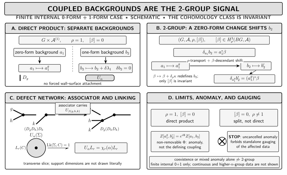
Panels A and B show that direct product requires $\rho=1$ and $[\beta]=0$; $[\beta]=0$ with nontrivial $\rho$ is split or semidirect, not direct. For a finite internal 2-group, panel C translates the Postnikov class into an operator statement: a wall associator carries a one-form symmetry surface, whose action is measured by a linked charged line in a stabilized sector. Panel D then separates that operator-valued decoration from a possible c-number anomaly and from the decision to gauge. The diagram is schematic and not to scale; its icons are transverse slices rather than literal support dimensions, junction existence and normalization are additional data, and RG flow is not depicted.

Swipe horizontally to inspect the complete comparison, or open the vector figure at full size.

The table gives the complete page-local nonvisual reading of the figure and extends it through gauging and RG flow.

Four consequences of the same coupled background data

Question	Required data	Licensed conclusion	Stop condition
Direct-product test	The action ρ and class [β]	Independent factors require trivial ρ and vanishing [β]	Vanishing [β] with nontrivial ρ is split or semidirect, not direct
Surface crossing	The action ρ	A wall transports surface labels and line characters	A scalar phase needs a stabilized one-dimensional character sector
Wall associator	A cocycle representative β and chosen binary junctions	The fusion-tree comparison carries a one-form surface	Its label does not construct the junction space
Full gauging	Constrained background pairs, gauge arrows, measure, and weights	Sum the complete two-group gauge groupoid	Anomaly, missing sectors, or boundary data can obstruct the sum
Partial gauging	A closed sub-two-group preserved by the action and Postnikov data	Gauge only that compatible substructure	An arbitrary factor or subgroup need not close
Charged line	Its higher charge and allowed attachments	A naked nonneutral line projects out or becomes attached	Projection is not dynamical screening
Dual symmetry	A finite Abelian gauged sector and its flux defects	Pontryagin-dual surfaces can measure new twisted sectors	The dual need not split from pre-existing symmetry
Anomaly	The full coupled transformation and allowed counterterms	An unremovable phase defines the obstruction class	The Postnikov class alone is not that phase
RG comparison	An exact background map from UV to IR	Structure and anomaly match up to the licensed equivalences	Breaking, emergence, kernels, or extensions change the comparison

Gaugeability belongs to the coupled background family

For a finite 2-group, a background is not an arbitrary pair of independent cocycles. It is a pair $(a,b)$ with

$$a\in Z^1(M;G), \qquad b\in C^2(M;\mathcal A_a), \qquad \delta_a b=a^*\beta,$$

modulo the coupled zero-form and one-form gauge arrows. Let $\operatorname{Bun}_{\mathbb G}(M)$ denote the resulting finite higher groupoid. When the full 2-group is anomaly-free and all global choices are fixed, its gauging has the schematic form

$$Z_{\mathcal T/\mathbb G}[M] = \sum_{[(a,b)]\in\pi_0\operatorname{Bun}_{\mathbb G}(M)} \mu_M[(a,b)]\, Z_{\mathcal T}[M;a,b]\,\Theta[a,b].$$

The measure $\mu_M$ contains automorphism and gauge-for-gauge factors; it is not a universal inverse of the number of topological sectors. $\Theta[a,b]$ is a separately chosen gauge-invariant topological weight. On a boundary, the background groupoid, measure, and weight require relative or boundary data rather than a copy of this closed-bulk formula.

Three different operations must not be conflated.

• Gauge the one-form part. A subgroup $K_1\subseteq\mathcal A$ must be preserved by the retained zero-form action, the complete anomaly must restrict trivially to $K_1$, and the constrained $b$ sectors must exist. The result can carry a dual symmetry and a mixed anomaly rather than a direct-product remnant.
• Gauge the zero-form part. If a zero-form gauge move forces $b$ to change, holding the one-form background fixed is not a gauge-covariant operation. One needs a compatible sub-2-group, a trivialization of the restricted Postnikov datum, or extra relative data.
• Gauge the full 2-group. Sum the pairs $(a,b)$ and their coupled gauge arrows together. Closure, anomaly cancellation, the higher-groupoid measure, tangential data, topological weights, singular defects, and boundary conditions are all inputs.

More generally, a partially gauged pair $(K_0,K_1)$ must itself define a sub-2-group: $K_1$ is stable under $K_0$, the restricted Postnikov class lands in the admitted $K_1$ data up to the allowed redefinitions, and the selected weights and boundary conditions preserve that structure. Ordinary subgroup closure alone does not establish gaugeability.

The general finite higher-form sum and its gaugeability tests are developed in the required gauging page. For higher groups specifically, the one-form-gauging obstruction and the conversion of Postnikov nonclosure into a dual mixed anomaly are summarized in Bhardwaj et al. 2024, § 5.2.3, arXiv v2, p. 121, eqs. (5.33)–(5.34), Open PDF.

Gauging transforms the operator network

Let $K_1$ be a finite Abelian one-form subgroup that passes the preceding tests. A line with character $\chi\in\widehat K_1$ meets the local character projector

$$\frac{1}{\lvert K_1\rvert} \sum_{k\in K_1}\chi(k) =\delta_{\chi,1}.$$

Hence a naked nonneutral line does not survive as a gauge-invariant genuine operator. If $C=\partial D$ and the background convention gives the line a positive gauge phase, the attached operator

$$L_\chi(C;D) :=L_\chi(C) \exp\!\left[-2\pi i \left\langle\chi(b),D\right\rangle\right]$$

is gauge invariant. The $(p+1)$-chain attachment is physical: changing $D$ by a closed cycle multiplies the insertion by a Wilson operator of the new dynamical higher gauge field. Neutral composites can survive without that attachment, but they still require endpoint, screening, and global-form checks.

The old $K_1$ symmetry surfaces become gauge redundancy. Defects that were twisted sectors can instead become genuine and charged under the new Pontryagin-dual symmetry. In four dimensions, gauging a finite one-form group $K_1$ produces a candidate dual one-form symmetry $\widehat K_1^{(1)}$ under the finite, Abelian, anomaly-free closed-bulk hypotheses. Its surfaces measure the new flux lines, and their fusion and junction incidence must be supplied just as in the original network.

This exchange of charged and twisted sectors is described in Bhardwaj et al. 2024, §§ 4.3.3–4.3.4, arXiv v2, pp. 88–92, eqs. (4.163)–(4.184) and fig. 18, Open PDF. It is a kinematic consequence of gauging; it does not decide screening dynamics, confinement, or the infrared phase.

Anomaly representatives are separate from the Postnikov class

Bundle the full coupled background into $\mathcal B=(a,b)$. Under a coupled gauge arrow $u$, an anomalous generating functional transforms as

$$Z_M[u\mathbin{\cdot}\mathcal B] = \exp\!\left(2\pi i\,\mathfrak A_M[\mathcal B;u]\right) Z_M[\mathcal B].$$

A local counterterm $C_M[\mathcal B]$ changes the representative by

$$\mathfrak A_M[\mathcal B;u] \longmapsto \mathfrak A_M[\mathcal B;u] +C_M[u\mathbin{\cdot}\mathcal B]-C_M[\mathcal B].$$

The anomaly is the equivalence class that remains after every allowed local counterterm. Its phase must satisfy the consistency condition obtained by composing coupled gauge arrows. By contrast, $[\beta]$ specifies those gauge arrows in the first place. The surface $U_{\beta(g,h,k)}$ in a wall associator is operator-valued; an anomalous phase in the network move is additional c-number data.

When a cohomological inflow representative exists, one may write on a $(d+1)$-manifold $X$ with boundary $M$

$$I_X[\mathcal B] =\exp\!\left( 2\pi i\int_X\omega_{d+1}(\mathcal B) \right),$$

whose boundary variation cancels the anomalous phase. This formula is a useful representative, not a universal classification: spin refinements, gravitational terms, torsion, and generalized-cohomology data can require a more general invertible field theory.

For finite internal bosonic 2-groups in the orientable setting, the defect phases, counterterm equivalences, and inflow analysis are developed in Benini, Córdova, and Hsin 2019, § 3, pp. 17–27, especially eqs. (3.19)–(3.37), Open PDF. That source explicitly does not make its treatment a classification of gravitational or spin-refined anomalies.

Renormalization-group comparisons require identified backgrounds

RG flow changes the dynamical description, but integrating out modes does not discard exact external probes. Suppose the UV 2-group is exact, the flow preserves it, and a map $f$ identifies the UV background groupoid with the backgrounds admitted by the intrinsic IR symmetry. Then the invariant comparison is

$$[\mathfrak A_{\mathrm{UV}}] =f^*[\mathfrak A_{\mathrm{IR}}],$$

up to local counterterms and invertible local factors. With the same faithful symmetry and global normalization on both sides, the action $\rho$ and Postnikov class $[\beta]$ likewise remain part of the background transformation law; a quantized structural class does not run continuously.

This statement is conditional in three important ways.

• The intrinsic IR symmetry can be larger than the UV symmetry. The UV background then couples through a homomorphism into the IR symmetry, and only the pulled-back IR anomaly is compared.
• If a subgroup acts trivially in the IR, the faithful quotient changes the presentation. One must compare after the kernel, extension, and background maps are stated, not equate group names.
• Spontaneous breaking, emergent symmetry, a decoupled topological sector, or relative bulk data can realize the same UV constraint without preserving the same microscopic operators.

A nonzero anomaly rules out a unique symmetric trivial gapped absolute IR under the usual locality and unitarity hypotheses. It can instead be matched by gapless degrees of freedom, symmetry breaking with its required topological terms, topological order, or a relative boundary theory. The anomaly does not choose among those possibilities.

The extrinsic-UV versus intrinsic-IR background map is explained in Benini, Córdova, and Hsin 2019, § 4, pp. 27–29, Open PDF. For continuous four-dimensional Abelian 2-groups, Córdova, Dumitrescu, and Intriligator 2019, § 1.5, pp. 14–15; § 4.4, pp. 44–47, especially eqs. (4.18)–(4.20), version-of-record PDF derives additional current-algebra constraints. Those inequalities depend on the stated continuous-current and CFT hypotheses; they are not universal finite-2-group theorems.

First application: gauge the electric ℤ₂ sector of a compact Abelian model

Before gauging: the SO(3)–ℤ₂ network

Work in Euclidean signature on a closed oriented spin four-manifold $M$, with the spin structure fixed and $\theta=0$. Let $\mathfrak a$ be a faithfully normalized compact $U(1)$ connection, $\mathfrak a\mapsto\mathfrak a+\mathrm d\lambda$ with $\lambda\sim\lambda+2\pi$, and let $f=\mathrm d\mathfrak a$ locally with

$$\frac{1}{2\pi}\int_{\Sigma_2}f\in\mathbb Z$$

on every closed oriented two-cycle. Take two complex scalars $\Phi=(\Phi_1,\Phi_2)$ of gauge charge $2$, with interactions preserving their flavor-doublet symmetry. Exclude odd-electric-charge endpoints, hold magnetic spectator backgrounds trivial, and keep dynamical monopoles outside this calculation.

For a closed oriented line $C$,

$$W_r(C)=\exp\!\left(i r\oint_C\mathfrak a\right), \qquad r\in\mathbb Z.$$

Charge-two matter screens $W_2$ while $W_1$ remains unscreened. The exact electric one-form symmetry is $\mathbb Z_2^{(1)}$. Let its surface be $U_s(\Sigma)$, $s\in\mathbb Z_2$. With $\mathcal X$ outside the sweep and closed, oriented, disjoint supports in a linking ball,

$$\left\langle U_s(\Sigma)W_r(C)\mathcal X\right\rangle =(-1)^{sr\operatorname{Lk}(\Sigma,C)} \left\langle W_r(C)\mathcal X\right\rangle.$$

The surfaces fuse as $U_s\otimes U_t\simeq U_{s+t}$. For two incoming sheets and one outgoing sheet meeting on an oriented line $K$, declare

$$I_{s,t}^{\ u}(K):U_s\otimes U_t\longrightarrow U_u, \qquad s+t-u=0\pmod 2$$

away from background sources. The congruence is necessary but does not construct or normalize the junction.

Gauge-invariant local operators see the faithful flavor group $SO(3)=SU(2)/\mathbb Z_2$. Retaining the flavor-center charge of allowed line endpoints refines the line group to

$$\widetilde{\mathcal D}_1 =\frac{\mathbb Z\times\mathbb Z_2}{\langle(2,1)\rangle} \cong\mathbb Z_4.$$

Let $P_f$ be an $SO(3)$ background. Choose cocycle representatives $w_2^f$ and $w_3^f=\operatorname{Bock}(w_2^f)$. The electric two-form background is a cochain $b_2$ obeying

$$\boxed{\delta b_2=w_3^f}.$$

Across a small transverse three-disk $D^3$ meeting a chosen representative of the source, the surface incidence becomes

$$s+t-u =\left\langle w_3^f,D^3\right\rangle \pmod 2.$$

Thus an otherwise forbidden odd incidence is allowed only at a declared background-sourced junction. The representative locus and its junction amplitude are not determined by the cohomology class alone.

This compact theory, its refined $\mathbb Z_4$ line group, and the constraint $\delta b_2=w_3^f$ are derived in Bhardwaj et al. 2024, examples 5.2 and 5.4, arXiv v2, pp. 123–129, eqs. (5.50)–(5.94), Open PDF.

Sum the constrained two-form field

Gauge the electric $\mathbb Z_2^{(1)}$ only after assuming that its restriction of the full higher-group anomaly vanishes and choosing the untwisted weight. For a compatible $SO(3)$ background with $[w_3^f]=0$, let $\mathscr S(P_f)$ be the affine set of gauge-equivalence classes of solutions to $\delta b_2=w_3^f$. Couple a closed dual background $\widehat b_2\in Z^2(M;\mathbb Z_2)$. In the standard one-form homotopy-cardinality convention,

$$\begin{aligned} Z_{\mathrm{gauged}}[M;P_f,\widehat b_2] ={}&\frac{\lvert H^0(M;\mathbb Z_2)\rvert} {\lvert H^1(M;\mathbb Z_2)\rvert} \\ &\times \sum_{[b_2]\in\mathscr S(P_f)} Z[M;P_f,b_2] (-1)^{\int_M\widehat b_2\smile b_2}. \end{aligned}$$

The sum is affine rather than a sum over an independent $H^2$ label. If $[w_3^f]\neq0$, no global ordinary $b_2$ solves the constraint on closed $M$, so this absolute formula is not available. Arbitrary obstructed flavor backgrounds require local or relative cocycles and the inflow description below; an empty sum must not be presented as a complete gauged theory.

On a small link of $W_r$, the exact gauge projector is

$$\frac12\sum_{s=0}^{1}(-1)^{sr} =\delta_{r\bmod2,0}.$$

Thus naked $W_1$ is non-genuine after gauging. If $C=\partial D$, the surface-attached line

$$W_r(C;D) :=W_r(C)(-1)^{r\langle b_2,D\rangle}$$

is gauge invariant. The neutral line $W_2$ survives this projection but was already screenable by the scalars; projection and screening remain different tests.

After gauging: dual surfaces and a mixed anomaly

The old $U_s$ sheets are now gauge transformations. Locally one may write

$$\mathfrak a'=2\mathfrak a, \qquad W_2(\mathfrak a)=W_1(\mathfrak a'),$$

so the matter has unit charge in the primed normalization. Although $U(1)/\mathbb Z_2\cong U(1)$ abstractly, the quotient admits fluxes that are half-integral in the old unit. This normalization change and the associated Wilson-lattice restriction follow from Gaiotto et al. 2015, § 4.1, arXiv v2, pp. 14–18, especially p. 16, eq. (4.3), Open PDF.

Away from the flavor-background source, the dual surface and a flux line can be represented by

$$\widehat U_t(\Sigma) :=(-1)^{t\langle b_2,\Sigma\rangle}, \qquad \left\langle b_2,S^2_{\mathrm{link}}\right\rangle=m\pmod2,$$

where $t,m\in\mathbb Z_2$ and the second equation defines $\widehat T_m(C')$. Their linked correlator is

$$\begin{aligned} \left\langle \widehat U_t(\Sigma)\widehat T_m(C')\mathcal X \right\rangle ={}&(-1)^{tm\operatorname{Lk}(\Sigma,C')} \\ &\times \left\langle\widehat T_m(C')\mathcal X\right\rangle. \end{aligned}$$

Dual surfaces fuse additively. A declared two-in/one-out dual junction $\widehat I_{s,t}^{\ u}(K)$ obeys $s+t-u=0\pmod2$ away from the flavor source. With no monopoles, this dual $\mathbb Z_2^{(1)}$ is the flux-parity subgroup or repackaging of the magnetic $U(1)^{(1)}$ data, not an independent factor that may be multiplied onto it without checking the extension and background conventions.

The Postnikov constraint now produces an anomaly under a dual one-form gauge move $\widehat b_2\mapsto\widehat b_2+\delta\widehat\lambda_1$:

$$\begin{aligned} (-1)^{\int_M\delta\widehat\lambda_1\smile b_2} &=(-1)^{\int_M\widehat\lambda_1\smile\delta b_2} \\ &=(-1)^{\int_M\widehat\lambda_1\smile w_3^f}. \end{aligned}$$

This phase is independent of the affine $b_2$ sector, so the full partition function obeys

$$Z_{\mathrm{gauged}}[\widehat b_2+ \delta\widehat\lambda_1] = (-1)^{\int_M\widehat\lambda_1\smile w_3^f} Z_{\mathrm{gauged}}[\widehat b_2].$$

The cup-product order is fixed as displayed; signs are immaterial modulo two. The four-dimensional phase is cancelled by the five-dimensional inflow

$$I_5[P_f,\widehat b_2] :=(-1)^{\int_{X_5}\widehat b_2\smile w_3^f}, \qquad \partial X_5=M,$$

when the backgrounds and required structures extend. The degrees check: $1+3=4$ in the boundary variation and $2+3=5$ in the inflow. Equivalently, moving a dual surface through a three-chain $V^3$ gives

$$\widehat U_1(\Sigma+\partial V^3) =(-1)^{\langle w_3^f,V^3\rangle} \widehat U_1(\Sigma).$$

Gauging has therefore traded the original Postnikov nonclosure for a mixed $SO(3)$–dual-$\mathbb Z_2^{(1)}$ ’t Hooft anomaly. The general conversion is given in Bhardwaj et al. 2024, § 5.2.3, arXiv v2, p. 121, eqs. (5.33)–(5.34), Open PDF. Pulling the flavor background back to $SU(2)$ sets $w_2^f$ and hence this $w_3^f$ to zero, but that changes the admitted symmetry background. It is not a local counterterm cancellation and does not prove that every anomaly of the lifted theory vanishes.

Any symmetry-preserving infrared description that retains the faithful $SO(3)$ and dual $\mathbb Z_2^{(1)}$ backgrounds must reproduce this mixed class. It may do so through gapless modes, symmetry breaking, topological order, or a relative bulk; the calculation does not select one of them.

What the four tests establish—and what they do not

The operator test is stronger than label coexistence. It records how walls transport one-form charges and how the Postnikov class decorates their associator. It does not make every line simple or every junction unique.

Gaugeability is a property of a background subfamily. A factor can be gauged only if its backgrounds close under the coupled transformations, its anomaly restriction vanishes, and its global measure, weights, boundaries, and attachments are defined. A formal subgroup symbol is insufficient.

Anomaly matching is a constraint, not a solution of dynamics. A nonzero class excludes a symmetric trivial gapped absolute endpoint under its stated hypotheses. It does not decide which permitted gapless, broken, topological, or relative realization occurs.

Current scope matters. In the narrower setting of $(2+1)$-dimensional Abelian bosonic TQFTs, a 2026 theorem proves that the time-reversal $H^3$ obstruction vanishes and reports no general proof covering arbitrary finite unitary groups $G$. That antiunitary result neither removes the four-dimensional Postnikov datum used here nor licenses every formal finite 2-group as a realized QFT. It supplies a useful contrary scope check Orii 2026, introduction, pp. 1–2, eqs. (1.1)–(1.4), version-of-record PDF.

Categorical and generalized-cohomology classification is outside this page. The formulas above are operational finite-QFT tests. They do not classify all higher groups, higher representations, spin anomalies, or relative field theories.

Common pitfalls

Calling the Postnikov surface an anomaly. The surface in the wall associator is operator-valued symmetry structure. An anomaly is an unremovable c-number phase under the complete coupled transformation.

Gauging a factor while freezing the field it must transform. If a zero-form gauge move shifts the two-form background, the proposed operation is not gauge covariant. Restrict to a compatible sub-2-group or supply the required relative completion.

Calling projection screening. Gauge averaging removes a naked charged operator from the gauge-invariant algebra. Screening instead requires an actual dynamical endpoint in the matter spectrum.

Adding the dual symmetry as an automatic direct factor. The dual can participate in an extension or mixed anomaly and can repackage a pre-existing magnetic sector. Determine the faithful action and global background before writing a product.

Writing the constrained sum on every flavor bundle. A global solution of $\delta b_2=w_3^f$ requires $[w_3^f]=0$. Obstructed backgrounds need the relative inflow description, not an ordinary empty or ill-defined sum.

Treating anomaly matching as a phase diagram. Matching removes inconsistent endpoints; it does not rank the remaining dynamical options.

Check your understanding

These checks test the page’s four operational consequences.

1. Transport a character.

If $\rho(g)$ sends $\alpha$ to $\rho(g)\alpha$, what character labels the line after crossing $D_g$?

The contragredient character is

$$(g\mathbin{\cdot}\chi)(\alpha) =\chi\!\left(\rho(g^{-1})\alpha\right).$$

Only when this equals $\chi$ may the wall action be collapsed to a scalar in that one-dimensional sector.

2. Test a proposed partial gauging.

Why is $K_0\subset G$ alone not enough to gauge the zero-form factor?

The zero-form gauge move can transport $\mathcal A$ and shift $b$ through the restricted Postnikov datum. A valid operation needs a compatible $K_1$, a closed sub-2-group, an anomaly-free restriction, and the corresponding global measure and boundary data. Freezing $b$ generally breaks gauge covariance.

3. Change an anomaly representative.

What does a local counterterm $C_M[\mathcal B]$ change?

It shifts $\mathfrak A_M[\mathcal B;u]$ by $C_M[u\cdot\mathcal B]-C_M[\mathcal B]$. Therefore a displayed phase is not itself invariant; only its equivalence class after all allowed counterterms is the anomaly.

4. Separate projection from screening.

In the compact model, compare $W_1$ and $W_2$ after gauging the electric $\mathbb Z_2^{(1)}$.

The character average kills naked odd charge, so $W_1$ needs a dynamical surface attachment. $W_2$ is neutral under the gauged $\mathbb Z_2$ and passes the projector, but charge-two scalar matter already supplies its endpoint. The first statement is projection; the second is screening.

5. Derive the dual anomaly.

Apply $\widehat b_2\mapsto\widehat b_2+\delta\widehat\lambda_1$ to the Fourier kernel. Which phase remains?

Cochain Stokes on closed $M$ and $\delta b_2=w_3^f$ give

$$(-1)^{\int_M\delta\widehat\lambda_1\smile b_2} =(-1)^{\int_M\widehat\lambda_1\smile w_3^f}.$$

It is cancelled by the boundary variation of $(-1)^{\int_{X_5}\widehat b_2\smile w_3^f}$. This is the mixed anomaly after gauging, not the original Postnikov class.

6. State the RG conclusion precisely.

What can be concluded if the exact UV and IR background families are identified and the mixed anomaly is nonzero?

Their anomaly classes agree up to local counterterms and the declared background map. A unique symmetric trivial gapped absolute IR is excluded under the standard locality and unitarity hypotheses, but gaplessness, symmetry breaking, topological order, or a relative bulk can match the class. No unique phase follows.

Continue to Symmetry TFT, mathematical classification, and model dynamics

Symmetry TFT: Encoding Symmetry, Anomaly, and Gauging is the next physical synthesis: it will organize symmetry defects, anomaly inflow, and alternative gauging choices as boundary data of a higher- dimensional topological theory.

For theorem-first higher representations and charge sectors, continue to Categorical Symmetries, Higher Representations, and Charges. Anomaly and Generalized-Symmetry Constraints on Infrared Phases is the destination for model-dependent infrared exclusions, while Symmetry Fractionalization and Projective Quantum Numbers treats microscopic and quasiparticle realizations.

The next chapter begins with Non-Invertible Topological Defects and Fusion, where the group-like inverse assumed throughout this page is no longer available.

References

• Benini, Francesco, Clay Córdova, and Po-Shen Hsin. “On 2-Group Global Symmetries and Their Anomalies.” Journal of High Energy Physics 2019, no. 3 (2019): 118. DOI. Open PDF.

• Bhardwaj, Lakshya, Lea E. Bottini, Ludovic Fraser-Taliente, Liam Gladden, Dewi S. W. Gould, Arthur Platschorre, and Hannah Tillim. “Lectures on Generalized Symmetries.” Physics Reports 1051 (2024): 1–87. DOI. Open PDF, arXiv v2.

• Córdova, Clay, Thomas T. Dumitrescu, and Kenneth Intriligator. “Exploring 2-Group Global Symmetries.” Journal of High Energy Physics 2019, no. 2 (2019): 184. DOI. Version-of-record PDF.

• Gaiotto, Davide, Anton Kapustin, Nathan Seiberg, and Brian Willett. “Generalized Global Symmetries.” Journal of High Energy Physics 2015, no. 2 (2015): 172. DOI. Open PDF, arXiv v2.

• Orii, Ippo. “Vanishing of the $H^3$ Obstruction for Time-Reversal Symmetry in $(2+1)$D Abelian Bosonic TQFTs.” Journal of High Energy Physics 2026, no. 3 (2026): 018. DOI. Open version-of-record PDF.