Renormalization and Effective Field Theory

Renormalization and effective field theory make quantum field theory predictive when a calculation probes more scales than one description can treat equally well. The central task is not to “remove infinities.” It is to declare an observable, degrees of freedom, scales, and approximation order, then state what is fitted, what runs, what is matched, what is invariant, what is omitted, and how that omission is tested.

This volume separates operations that are often compressed into the word scale: regulating an intermediate expression, choosing renormalized inputs, varying a subtraction scale, integrating out modes, matching descriptions, factorizing momentum regions, and truncating an expansion. Once those operations are kept distinct, locality, symmetry, renormalization-group invariance, and power counting become practical checks rather than slogans.

Helpful background. The volume assumes the distinction between an auxiliary regulator and a physical cutoff developed in Regulators, Cutoffs, and Continuum Limits, the separation of ultraviolet and infrared poles used in UV/IR Poles and the Renormalized-Amplitude Interface, the insertion language of Local and Composite Operator Insertions, and the quantum symmetry qualifications in Quantum Currents, Improvements, and Conservation. These are helpful rather than universal prerequisites: the routing guide below identifies the smallest repair for each starting point.

Seven operations that must not be conflated

A regulated amplitude may contain a parameter such as $\epsilon$ , $\Lambda_{\rm UV}$ , or a lattice spacing. A renormalized description introduces parameters defined by conditions or a subtraction prescription. Renormalization-group running compares those renormalized descriptions as an arbitrary scale $\mu$ changes while the bare theory—or, more generally, the physical prediction—is held fixed. Wilsonian flow instead changes the action because a band of fluctuations has been integrated out. Matching changes the active degrees of freedom. Factorization separates modes that coexist in the same observable. Power counting orders the terms that remain.

These operations can appear in a single calculation, but their invariants and failure tests differ. The local counterterm theorem concerns regulator removal; an RG equation concerns independence from an arbitrary scale; a matching equation concerns equality of two descriptions in their shared low-energy domain. Collins develops the first three distinctions directly in perturbation theory, while Wilson–Kogut and Polchinski formulate coarse graining as motion through theory space Collins 1984/2023, chs. 5–8, pp. 88–243 Wilson and Kogut 1974, §§ 3–12, pp. 94–175 Polchinski 1984, §§ 2–4, pp. 271–293.

Operation	What changes	What is held fixed or compared	Decisive check
Regularization and removal	Intermediate propagators, measures, dimensions, or domains	Renormalized inputs and the target observable	The removal limit exists after allowed local counterterms, with required identities restored
Subtraction and $\mu$ -running	Renormalized parameters, fields, operators, and coefficients	Bare quantities or the complete prediction	Residual $\mu$ dependence starts beyond the retained order
Wilsonian coarse graining	The action or effective average action at scale $k$	The partition function and long-distance observables	The flow closes in theory space; projection and truncation errors are exposed
Threshold matching	Degrees of freedom and Wilson coefficients	Full- and effective-theory amplitudes in their common infrared regime	Shared infrared terms cancel from the extracted short-distance coefficient
Factorization and rapidity evolution	Mode-separated functions and, when needed, a rapidity scale $\nu$	Their convolution or product in the observable	Virtuality and rapidity consistency equations cancel auxiliary-scale dependence
Approximation and truncation	The retained orders in couplings, derivatives, $1/M$ , velocities, or other expansion parameters	The declared domain and observable	The next omitted order is estimated and tested against order-by-order behavior
Change of scheme or basis	Coordinates used for couplings and operators	Predictions after finite parameter and coefficient maps	The transformed result agrees through the claimed order

The diagram is a routing map, not an energy-axis plot. Read each row horizontally: the arrow names an operation, and the right-hand box states the invariant or error test that licenses it. Its dashed arrows mark typed connections to prerequisite or application material in other volumes.

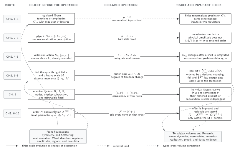
Six scale-changing operations map regulated descriptions, renormalized parameters, Wilsonian actions, full theories, factorized modes, and EFT truncations to different invariants and tests; finite scheme or basis changes supply a seventh, coordinate-changing operation. — Scale-flow map for the volume. The six rows show operations that change a scale, field content, or approximation order. Finite scheme and basis transformations—the seventh operation in the table—change coordinates at fixed physics and are therefore explained alongside the map rather than drawn as another scale-flow row. Dashed arrows show typed cross-volume connections. The diagram is schematic and not to scale.

Two warnings organize everything that follows. First, a vanishing regulator is not the same limit as $\mu\to\infty$ or $k\to0$ . Second, a formally exact parent equation does not make a projected or truncated solution exact. The functional-RG review by Dupuis and collaborators is especially explicit about the approximation schemes needed to turn an exact flow equation into numbers Dupuis et al. 2021, § 2.

Choose the chapter by the question

Start from the operation you need to perform, not from a preferred formalism.

If the immediate question is…	Begin with…	Leave with…
Which subgraphs diverge, and why are the subtractions local?	Ultraviolet Renormalization and Locality	A regulator-removal argument with forest recursion, symmetry conditions, and a finite-input map
How do insertions mix, including contact terms and basis dependence?	Composite Operators and Mixing	A closed operator sector and dual coefficient evolution with signs and transposes fixed
How does a finite prediction reorganize as $\mu$ changes?	Renormalization-Group Equations and Running	Coupled RG equations, invariants, improved logarithms, and a scheme-covariance check
What does it mean to integrate out fluctuations continuously?	Wilsonian and Functional Renormalization	A theory-space flow, an exact functional equation, and an explicit projection-error contract
Which flow directions and exponents are universal?	Fixed Points, Universality, and Continuum Limits	A stability analysis whose continuum-limit claim is bounded by the available evidence
Which operators belong in a low-energy theory, and to what order?	Effective Field Theory: Construction and Power Counting	A declared domain, degrees of freedom, counting rule, loop-closure test, and truncation estimate
How are short-distance coefficients determined across a threshold?	Matching, Decoupling, and Threshold Evolution	A full-minus-effective extraction with shared-infrared cancellation and a residual-scale test
When are two operator lists physically equivalent?	Operator Bases and Field Redefinitions	A quotient construction with flavor, Fierz, evanescent, and translation metadata
How are several low scales separated without double counting?	Modes, Factorization, and Multiscale RG	A mode table, multipole expansion, overlap prescription, factorized operator, and compatible $\mu$ / $\nu$ evolution
Which EFT architecture fits the scale hierarchy at hand?	Effective-Theory Architecture Atlas	A bounded framework card and a direct route to its applications
What can scale sensitivity, tuning, or emergence actually establish?	Naturalness, Scale Sensitivity, and Emergence	A separation of calculable corrections, coordinate choices, priors, and explanatory judgment

If a problem involves more than one row, preserve the order of dependencies. For example, a heavy-particle observable normally needs an EFT domain and counting rule before matching, matching before threshold running, and all ingredients before a residual-scale or truncation test. Appelquist and Carazzone establish decoupling only under stated low-momentum and renormalization assumptions; “heavy fields decouple” is therefore a conclusion to test, not an instruction to delete them Appelquist and Carazzone 1975, pp. 2856–2861.

Check your preparation

Try the task relevant to your route; if it stalls, use the linked review page and return.

Task	Ready when you can…	Smallest repair
Read a regulated loop result	Identify which singular terms are ultraviolet, infrared, or mixed, without inferring the answer from a scaleless integral alone	UV/IR Poles and the Renormalized-Amplitude Interface
Renormalize a local insertion	Explain why coincident insertions require new local data beyond separated-point correlators	Local and Composite Operator Insertions
Enforce a quantum symmetry	State the functional identity to be preserved and distinguish an anomaly from a removable breaking	Quantum Currents, Improvements, and Conservation
Build an EFT	Name the active fields, hierarchy, observable, expansion parameter, and proposed failure scale	Effective Field Theory: Construction and Power Counting
Linearize an RG flow	Diagonalize or Jordan-reduce a stability matrix and declare whether flow is toward the infrared or ultraviolet	Fixed Points, Universality, and Continuum Limits
Translate an operator basis	Track the coefficient map contragrediently when operators are changed	Operator Bases and Field Redefinitions

A correct numerical loop integral is not yet a renormalized prediction. Conversely, a reader need not master every regularization method before using EFT power counting. What matters is the ability to state the object being changed and the invariant being tested.

Four interacting routes through the volume

The chapters form four trunks, with deliberate crossings between them.

Local renormalization

Ultraviolet Renormalization and Locality moves from superficial degree and subdivergences to local counterterms, renormalized rules, physical inputs, regulator removal, and scheme maps. Stop if the proposed subtraction is nonlocal or if the removal limit has not been shown.
Composite Operators and Mixing treats insertions as their own renormalization problem, including contact products and matrix evolution. Stop if the operator sector is not closed under the symmetries and working order.
Renormalization-Group Equations and Running derives scale equations from fixed bare data, then separates scheme-dependent trajectories from invariant predictions. Stop if running parameters are presented without the compensating observable dependence.

Theory-space flow

Wilsonian and Functional Renormalization constructs momentum-shell and functional flows and distinguishes an exact flow equation from its projection. Stop if regulator or ansatz dependence is hidden.
Fixed Points, Universality, and Continuum Limits turns fixed points into stability data, exponents, crossover laws, and evidence-qualified continuum claims. Stop if a beta-function zero is treated as a complete QFT.

Controlled effective descriptions

Effective Field Theory: Construction and Power Counting defines domains, active fields, local expansions, counting, promoted interactions, and breakdown tests. Stop if no expansion parameter or closure check is declared.
Matching, Decoupling, and Threshold Evolution extracts short-distance data and evolves it between thresholds. Stop if full and effective descriptions do not share the same infrared convention.
Operator Bases and Field Redefinitions constructs the physical quotient and makes translations reproducible. Stop if an EOM, integration-by-parts, flavor, evanescent, or on-shell qualification is implicit.

Multiscale architecture and interpretation

Modes, Factorization, and Multiscale RG derives mode-separated descriptions with overlap control and coupled evolution. Stop if a region is promoted to a mode without a homogeneous scaling and interaction analysis.
Effective-Theory Architecture Atlas compares reusable EFT structures without replacing their application volumes. Stop at the card boundary and follow the linked subject page for coefficients or phenomenology.
Naturalness, Scale Sensitivity, and Emergence separates technical calculations from interpretive claims. Stop if a regulator-dependent term, a coordinate-dependent tuning measure, and an observable sensitivity are being treated as the same evidence.

The local and Wilsonian trunks are complementary rather than rival definitions. Perturbative renormalization is efficient near a chosen action and observable; Wilsonian flow displays how all symmetry-allowed interactions are organized under changes of resolution. EFT uses both: locality controls its operator expansion, and RG flow transports its coefficients between scales. Manohar gives a compact derivation of this logic from matching through running and power counting Manohar 2018, §§ 3–7, pp. 11–61.

Six examples that connect the chapters

Following one object across chapters is often more useful than reading every formalism in isolation.

Thread	Construction	Cross-check	Continue with
Scalar renormalized prediction	Degree count $\to$ regulator $\to$ forests $\to$ local counterterms $\to$ renormalized inputs	Regulator removal and finite scheme map	A model-specific observable in Scattering or Many-Body Quantum Matter
Operator running	Insertion $\to$ contact terms $\to$ mixing matrix $\to$ anomalous dimension $\to$ dual coefficient evolution	Basis covariance and scale cancellation in $C_iO_i$	A named operator sector in Gauge Theories and the Standard Model or nonperturbative step scaling in Lattice and Hamiltonian Field Theory
RG continuum limit	Bare independence $\to$ beta functions $\to$ theory-space flow $\to$ stability matrix $\to$ exponents	Regulator, truncation, and evidence review	Fixed-point observables in Conformal Field Theory and the Bootstrap or rigorous control in Mathematical Quantum Field Theory
Heavy-mediator EFT	Domain $\to$ local expansion $\to$ counting $\to$ matching $\to$ threshold running	Shared-infrared cancellation and residual matching-scale independence	A named weak, strong, flavor, or gravity application
Multiscale factorization	Regions $\to$ modes $\to$ multipole expansion $\to$ overlap subtraction $\to$ factorized operator $\to$ $\mu$ / $\nu$ evolution	Cancellation of both auxiliary scales in the observable	A process-level factorization theorem in Scattering or Gauge Theories and the Standard Model
Unstable resonance	Complex-pole input $\to$ width hierarchy $\to$ resonant field $\to$ nonresonant operators $\to$ hard matching	Gauge-invariant matched amplitude and controlled $\Gamma/M$ counting	Pole and line-shape observables in Scattering

Each thread has a failure mode worth preserving. Local counterterms can fail to respect a symmetry unless the correct functional identity is imposed. Operator evolution can appear to disagree because coefficients were not transformed contragrediently. A fixed point can be a truncation artifact. A matching coefficient can inherit spurious infrared dependence. A factorized expression can double count an overlap. A resonance expansion can lose gauge invariance if the pole hierarchy is imposed only on selected diagrams.

Convention card for scales, operators, and matching

The site-wide metric and Fourier conventions apply. This volume adds the following scale and matrix conventions where needed.

Dimensional regularization and subtraction

Unless a page states otherwise, perturbative dimensional regularization uses

d=4-2\epsilon.

The symbol $\mu$ denotes a renormalization scale, not a Wilsonian cutoff. Minimal subtraction (MS) removes pole terms in $\epsilon$ ; modified minimal subtraction ( $\overline{\rm MS}$ ) also absorbs the standard $\ln 4\pi-\gamma_E$ convention. A page that compares schemes must state the finite parameter map, because a named subtraction prescription alone does not define the physical inputs.

For a renormalized coupling $g^a(\mu)$ ,

\beta^a(g) \equiv \left.\mu\frac{d g^a}{d\mu}\right|_{g_0},

where the derivative is taken at fixed bare data. A truncated beta function and its zeros are scheme coordinates; observables and properly qualified critical data carry the invariant content.

Operator and coefficient orientation

Pages that use matrix mixing adopt column vectors of renormalized operators and write

O_i^{(0)}=Z_{ij}O_j, \qquad \gamma\equiv Z^{-1}\mu\frac{dZ}{d\mu}.

Fixed bare operators then imply

\mu\frac{dO}{d\mu}=-\gamma O.

For an effective interaction $\mathcal L_{\rm eff}=C^T O$ , scale independence requires the dual evolution

\mu\frac{dC}{d\mu}=\gamma^T C.

A source using the opposite sign for $\gamma$ , row-vector operators, or $O=Z O^{(0)}$ is not inconsistent; it uses a different convention. Translate the defining equation before comparing entries of an anomalous-dimension matrix.

Wilsonian and functional flows

A Wilsonian action $S_k$ and an effective average action $\Gamma_k$ are different functionals. The scale $k$ labels which fluctuations have been integrated out or suppressed, and the page must state whether the flow is read from ultraviolet to infrared or in the reverse direction. “Relevant” and “irrelevant” are incomplete labels without that direction and the chosen fixed point. An exact flow for a functional becomes an approximate result after an ansatz, regulator choice, derivative expansion, vertex truncation, or numerical discretization; convergence across controlled enlargements is part of the evidence.

Matching and uncertainty

At a matching scale $\mu_M$ near a heavy threshold $M$ , coefficients are defined so that full and effective descriptions agree for the declared low-energy external states and kinematics:

\mathcal A_{\rm full} = \mathcal A_{\rm EFT} +\mathcal O\!\left((Q/M)^{n+1}\right).

Both sides must use compatible ultraviolet and infrared conventions. The Wilson coefficient is short-distance data only after the common infrared contribution cancels. Evolution away from $\mu_M$ resums logarithms; varying $\mu_M$ is a diagnostic of omitted orders, not a substitute for matching.

Every quantitative EFT claim should distinguish at least parametric uncertainty, perturbative or matching uncertainty, EFT truncation uncertainty, and numerical or regulator uncertainty when present. Correlations matter: adding every component in quadrature is not a convention that can be assumed silently. A breakdown estimate should be challenged by order-by-order behavior, alternative observables, and known nearby thresholds.

Connections to the rest of QFT.org

This volume develops reusable renormalization and EFT structure. It stops before model-specific dynamics or process phenomenology takes over.

Neighbor	This volume supplies	Continued there
Scattering Amplitudes and Observables	Local UV subtraction, running, matching, mode and coefficient organization	Integral reduction, expansion by regions as an integral method, process factorization, Sudakov calculations, resonance sheets, and measured observables
Gauge Theories and the Standard Model	General symmetry-compatible renormalization, bases, matching, and RG machinery	QED, QCD, and Standard Model coefficients, named operator sectors, processes, fits, and bounds
Nonperturbative Quantum Field Theory	Fixed-point and EFT interfaces; the renormalon/OPE ambiguity contract	Condensate dynamics, confinement, strong-coupling mechanisms, and nonperturbative completion
Lattice and Hamiltonian Field Theory	Continuum and operator-running targets	Discretized actions, improvement, Monte Carlo, finite-volume analysis, and production step scaling
Conformal Field Theory and the Bootstrap	Fixed-point stability and scaling exponents	Conformal representations, correlators, OPE data, crossing, and bootstrap constraints
Thermal and Nonequilibrium Field Theory	General matching and scale-separation grammar	Schwinger–Keldysh and KMS construction, transport, noise, dissipation, and open dynamics
Many-Body Quantum Matter	Reusable Wilsonian, fixed-point, and EFT architecture	Phase-specific collective dynamics and many-body applications
Quantum Field Theory in Curved Spacetime	General local EFT, matching, and running logic	Curvature-dependent renormalization and gravitational applications
Holography and Quantum Gravity	Scale-flow and EFT prerequisites	Holographic and quantum-gravity interpretation
Mathematical Quantum Field Theory	Perturbative and Wilsonian bridges	Theorem-first, axiomatic, and constructive control

When an application needs a coefficient, a fit, a bound, or a phase diagram, follow the linked application volume. When it needs the reason a coefficient exists, how it transforms, what scale equation it obeys, or how its uncertainty is organized, return here.

Practice, reproducible calculations, Research, and Reference

The Renormalization and EFT pathway for working researchers provides a shorter route through the volume. The core primers on loops and regularization, renormalization and RG, and effective field theory repair common entry gaps. Exercises in this volume test definitions, calculations, and transfer to nearby problems; worked solutions make them suitable for self-study.

Numerical experiments on renormalization schemes, operator mixing and evolution, RG flows and fixed points, functional RG, EFT power counting and matching, operator bases, and unstable-particle EFT should publish their environment, inputs, and checks with the implementation. The pages here explain the benchmarks and analytic checks needed to interpret those computations.

Use Research for dated comparisons, datasets, and claims whose evidential state can change. Use the Reference hub for stable conventions, formulas, notation, and compact translations. The expository pages in this volume remain self-contained for their declared scope: those hubs extend or operationalize the reasoning; they do not replace it.

What you should be able to do

After the relevant chapters, you should be able to produce an object that another calculation can inspect:

a finite prediction with its regulator-removal and symmetry checks;
a closed operator sector with a reproducible anomalous-dimension and coefficient convention;
an RG solution whose invariant content and approximation order are explicit;
a fixed-point claim accompanied by a stability matrix and an evidence grade;
an EFT specification with domain, fields, counting, closure, uncertainty, and breakdown tests;
a matching analysis showing shared-infrared cancellation and residual scale independence;
an operator-basis translation that preserves physical amplitudes and records all qualifications; or
a multiscale factorization analysis with modes, overlap control, and compatible auxiliary-scale evolution.

The common standard is simple to state and demanding to meet: the output must say what changes, what does not, why the approximation is controlled, and what observation would show that it has failed.

References

Appelquist, Thomas, and J. Carazzone. 1975. “Infrared Singularities and Massive Fields.” Physical Review D 11: 2856–2861. DOI.
Collins, John C. 1984; open-access reissue 2023. Renormalization: An Introduction to Renormalization, the Renormalization Group and the Operator-Product Expansion. Cambridge Monographs on Mathematical Physics. Cambridge University Press. DOI and Open PDF.
Dupuis, Nicolas, Léonie Canet, Astrid Eichhorn, Walter Metzner, Jan M. Pawlowski, Michel Tissier, and Nicolás Wschebor. 2021. “The Nonperturbative Functional Renormalization Group and Its Applications.” Physics Reports 910: 1–114. arXiv:2006.04853.
Manohar, Aneesh V. 2018. “Introduction to Effective Field Theories.” Les Houches lecture notes. arXiv:1804.05863.
Polchinski, Joseph. 1984. “Renormalization and Effective Lagrangians.” Nuclear Physics B 231: 269–295. DOI.
Wilson, Kenneth G., and John Kogut. 1974. “The Renormalization Group and the $\epsilon$ Expansion.” Physics Reports 12: 75–199. DOI.