Gaussian and Wilson–Fisher Fixed Points

The Wilson–Fisher fixed point is the canonical example of an interacting continuum theory obtained by perturbing away from an upper critical dimension. In $d=4-\epsilon$, the quartic scalar interaction changes from marginal to relevant at the Gaussian point, while its one-loop self-interaction produces a nearby nonzero zero of the beta function. Tuning the mass then yields an infrared critical theory whose exponents can be expanded systematically in $\epsilon$.

Required background. Fixed Points and Linearized RG Flow fixes the stability convention, and Beta Functions, Mass Running, and Field Anomalous Dimensions supplies the renormalization-group identities. Helpful background. Asymptotic Scales, Remainders, Uniformity, and Optimal Truncation clarifies the status of a truncated epsilon expansion, while Saddles and the Semiclassical Expansion reviews scalar stability and loop organization.

The O(N) scalar theory below four dimensions

Let $\phi^a$, $a=1,\ldots,N$, be a real $O(N)$ vector and define

$$\rho\equiv\frac12\phi^a\phi^a.$$

In Euclidean signature, use the renormalized Lagrangian

$$\mathcal L = \frac12 Z_\phi(\partial_\mu\phi^a)^2 +m^2\rho +\mu^\epsilon\frac{\lambda}{6}\rho^2, \qquad d=4-\epsilon.$$

Since $\rho^2=(\phi^a\phi^a)^2/4$, the interaction is the standard $\mu^\epsilon\lambda(\phi^2)^2/4!$. The factor $\mu^\epsilon$ makes the renormalized $\lambda$ dimensionless. We will use

$$g\equiv\frac{\lambda}{8\pi^2}.$$

At the free fixed point, $\Delta_\phi=(d-2)/2$ and the quartic operator has coupling exponent

$$\theta_{\phi^4}=4-d=\epsilon.$$

Thus the interaction is relevant under infrared coarse graining when $\epsilon>0$, marginal at $d=4$, and irrelevant for $d>4$. This canonical term alone cannot produce a nonzero fixed point; the loop correction is essential.

One-loop beta functions

The one-loop four-point diagrams in the three crossing channels combine with the $O(N)$ index contractions to give the factor $N+8$. Minimal subtraction may be summarized by

$$\lambda_0 = \mu^\epsilon \left[ \lambda +\frac{N+8}{48\pi^2\epsilon}\lambda^2 +O(\lambda^3) \right].$$

Holding the bare coupling fixed gives

$$\beta_\lambda \equiv \mu\frac{d\lambda}{d\mu} = -\epsilon\lambda +\frac{N+8}{48\pi^2}\lambda^2 +O(\lambda^3).$$

In the chapter normalization,

$$\boxed{ \beta_g =-\epsilon g +\frac{N+8}{6}g^2 +O(g^3) }.$$

The one-loop two-point tadpole renormalizes the mass but has no momentum dependence, so

$$m_0^2 =m^2 \left[ 1+\frac{N+2}{48\pi^2\epsilon}\lambda +O(\lambda^2) \right], \qquad Z_\phi=1+O(\lambda^2).$$

For the dimensionless temperature-like mass scaling field $\tau$, this yields

$$\partial_t\tau = \left[ -2+\frac{N+2}{6}g+O(g^2) \right]\tau +O(\tau^2),$$

where $t=\ln(k/\Lambda_{\mathrm{UV}})$. A momentum cutoff can add a scheme-dependent shift to the raw mass; $\tau=0$ means the nonlinear mass scaling field has been tuned to the critical surface, not that an arbitrary bare $m_0^2$ vanishes.

The field anomalous dimension begins at two loops because the one-loop self-energy has no external-momentum dependence:

$$\eta = \frac{N+2}{2(N+8)^2}\epsilon^2 +O(\epsilon^3).$$

The original epsilon-expansion construction and its diagrammatic organization are given in Wilson and Fisher 1972, pp. 240–243 and developed in Wilson and Kogut 1974, §§ 12–13, pp. 166–184.

Gaussian and interacting zeros

To the displayed order, $\beta_g=0$ has two solutions:

$$g_{\mathrm G}=0, \qquad \boxed{ g_{\mathrm{WF}} =\frac{6\epsilon}{N+8} +O(\epsilon^2) }.$$

For physical $N\geq1$ and small positive $\epsilon$, the interacting coordinate is positive and the quartic potential is bounded below. It merges with the Gaussian point as $\epsilon\to0^+$. Continuing to $\epsilon<0$ gives a negative formal zero at this order, outside the stable positive-coupling scalar theory.

The derivative of the beta function is

$$\beta_g'(g) =-\epsilon+\frac{N+8}{3}g+O(g^2).$$

At the Gaussian point,

$$B_g=-\epsilon, \qquad \theta_g^{\mathrm G}=\epsilon.$$

The quartic is relevant for $\epsilon>0$. At the Wilson–Fisher point,

$$B_g=+\epsilon+O(\epsilon^2), \qquad \boxed{ \theta_g^{\mathrm{WF}} =-\epsilon+O(\epsilon^2) }.$$

It has become irrelevant, with leading correction exponent $\omega=\epsilon+O(\epsilon^2)$. The mass direction remains relevant:

$$\boxed{ \theta_t =2-\frac{N+2}{N+8}\epsilon +O(\epsilon^2) }.$$

For $0<g<g_{\mathrm{WF}}$, $\beta_g<0$. Lowering $k$ means $dt<0$, so $dg=\beta_gdt>0$ and the flow moves toward $g_{\mathrm{WF}}$. For $g>g_{\mathrm{WF}}$ but still inside the perturbative neighborhood, the sign reverses and infrared flow again approaches the zero. This attraction occurs only in the quartic direction; the mass must still be tuned.

Panel (c) of the shared figure encodes these arrows. Panels (a) and (b) show the simultaneous mass tuning and decay of the quartic correction.

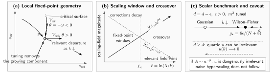
A fixed point organizes local flow, not every global trajectory. Panel (a) shows the critical surface tangent to the irrelevant eigendirection and the relevant departure under infrared flow. Panel (b) compares $e^{\theta\ell}$ growth with $e^{-\omega\ell}$ corrections for $\ell=\ln(\Lambda/k)$. Panel (c) shows the tuned one-loop $O(N)$ scalar trajectory from the Gaussian point to $g_\star=6\epsilon/(N+8)$ and the dangerously irrelevant-coupling exception to naive hyperscaling. The diagram is schematic and not to scale.

A reproducible calculation can plot this quadratic beta function and vary $N$ and $\epsilon$. Its perturbative curve should not be extrapolated past couplings where the omitted $O(g^3)$ term can compete with those retained.

Critical exponents to leading order

The correlation-length exponent follows from the thermal eigenvalue:

$$\nu =\frac{1}{\theta_t} =\frac12 +\frac{N+2}{4(N+8)}\epsilon +O(\epsilon^2).$$

Combining $\nu$ with $\eta=O(\epsilon^2)$ and expanding every scaling relation consistently gives

$$\begin{aligned} \alpha &=\frac{4-N}{2(N+8)}\epsilon +O(\epsilon^2),\\ \beta_{\mathrm{mag}} &=\frac12-\frac{3}{2(N+8)}\epsilon +O(\epsilon^2),\\ \gamma &=1+\frac{N+2}{2(N+8)}\epsilon +O(\epsilon^2),\\ \delta &=3+\epsilon+O(\epsilon^2),\\ \omega &=\epsilon+O(\epsilon^2). \end{aligned}$$

The order-parameter exponent is labeled $\beta_{\mathrm{mag}}$ to avoid confusion with $\beta_g$. The value of $\eta$ written earlier is already of second order; inserting it while dropping all other $O(\epsilon^2)$ contributions does not produce a consistently second-order exponent table.

For $N=1$ these formulas reduce to

$$g_{\mathrm{WF}}=\frac23\epsilon, \quad \nu=\frac12+\frac{\epsilon}{12}+O(\epsilon^2), \quad \eta=\frac{\epsilon^2}{54}+O(\epsilon^3), \quad \omega=\epsilon+O(\epsilon^2).$$

Setting $\epsilon=1$ in these leading terms illustrates the direction of the three-dimensional corrections, but it is not a controlled precision estimate: the formal small parameter is then order one.

There is a useful analytic check at large $N$. The result becomes

$$\nu =\frac12+\frac14\epsilon+O(\epsilon^2,N^{-1}),$$

which is the expansion of the leading large-$N$ value $\nu=1/(d-2)=1/(2-\epsilon)$. Also $\eta\to0$ as $N\to\infty$. These limits independently check the group factors and signs.

Coordinate and scheme dependence

The fixed-point coordinate $\,g_{\mathrm{WF}}$ is not itself an observable. Let an admissible scheme transformation be

$$g'=g+a g^2+O(g^3).$$

Then $\beta_{g'}=(dg'/dg)\beta_g$. The transformed fixed point has

$$g'_{\mathrm{WF}} =g_{\mathrm{WF}}+a g_{\mathrm{WF}}^2+\cdots,$$

so its coordinate changes at $O(\epsilon^2)$. At an exact fixed point the stability derivative transforms by similarity and its eigenvalue is invariant. At finite order, different schemes can disagree by terms beyond the retained order; that spread is an uncertainty diagnostic, not a new universal number.

The leading one-loop coefficients displayed here are sufficient for $g_{\mathrm{WF}}$ through $O(\epsilon)$ and for $\nu$ through $O(\epsilon)$. Quantitative work at $\epsilon=1$ requires higher-loop series, a declared resummation, and comparison with nonperturbative evidence. Le Guillou and Zinn-Justin demonstrate why resummation and large-order information matter in Le Guillou and Zinn-Justin 1980, §§ II–IV, pp. 3976–3998.

Wilsonian interpretation and limits

The epsilon expansion has a direct Wilsonian reading. At $d=4$, the Gaussian fixed point has a marginal quartic direction. Lowering the dimension gives that direction the small positive canonical exponent $\epsilon$. Loop fluctuations bend the flow and produce an interacting zero at $g=O(\epsilon)$. Because the fixed point is parametrically close to the Gaussian theory, both the beta function and the anomalous dimensions are perturbatively calculable.

The construction establishes a local fixed point and its expansion under the following conditions:

• $\epsilon$ is small enough that $g_{\mathrm{WF}}=O(\epsilon)$ is perturbative;
• the mass scaling field is tuned to the critical surface;
• the stable positive quartic branch is used;
• exponents and scaling relations are truncated at a common order;
• no additional relevant operator allowed by the chosen symmetry sector has been omitted.

It does not, at leading order, provide a precision exponent set in three dimensions, prove convergence of the epsilon series, classify every $N$ and dimension, or replace checks of reflection positivity and global RG trajectories. The next page, Ultraviolet and Infrared Fixed Points: Criteria and Evidence, generalizes those evidence requirements beyond this controlled benchmark.

Common pitfalls

Reading arrows from the sign of $\beta_g$ alone. Infrared evolution has $dt<0$. For $0<g<g_{\mathrm{WF}}$, a negative beta function therefore makes $g$ increase toward the fixed point.

Calling the Wilson–Fisher point fully IR-attractive. It is attractive in the quartic direction but has a relevant mass direction. Critical behavior requires mass tuning.

Treating $g_\star$ as universal. Coupling coordinates change under analytic scheme and field redefinitions. Stability exponents and properly normalized observables are the comparison targets.

Substituting $\epsilon=1$ without an error statement. A leading epsilon result at order-one epsilon is an extrapolation. Higher orders, resummation, and independent nonperturbative methods determine whether it is quantitatively reliable.

Exercises

1. Integrate the one-loop quartic flow

Solve $\partial_tg=-\epsilon g+A g^2$ with $A=(N+8)/6$ and initial value $g(t_0)=g_0$.

Solution

With $g_\star=\epsilon/A$, separation gives

$$\frac{g(t)}{g_\star-g(t)} = \frac{g_0}{g_\star-g_0} e^{-\epsilon(t-t_0)}.$$

Equivalently,

$$g(t) = \frac{g_\star} {1+\left(g_\star/g_0-1\right)e^{\epsilon(t-t_0)}}.$$

For $0<g_0<g_\star$ and $t\to-\infty$, the exponential vanishes and $g(t)\to g_\star$, confirming infrared attraction.

2. Derive the thermal exponent

Insert $g_{\mathrm{WF}}=6\epsilon/(N+8)$ into $\partial_t\tau=[-2+(N+2)g/6]\tau$ and obtain $\nu$ through first order.

Solution

At the fixed point,

$$B_\tau =-2+\frac{N+2}{N+8}\epsilon,$$

so $\theta_t=-B_\tau=2-(N+2)\epsilon/(N+8)$. Expanding its reciprocal,

$$\nu =\frac1{\theta_t} =\frac12 +\frac{N+2}{4(N+8)}\epsilon +O(\epsilon^2).$$

3. Verify the first-order scaling relations

Use the displayed $\alpha$, $\beta_{\mathrm{mag}}$, and $\gamma$ to check Rushbrooke’s relation through $O(\epsilon)$.

Solution

The $O(\epsilon)$ coefficient in $\alpha+2\beta_{\mathrm{mag}}+\gamma$ is

$$\frac{4-N}{2(N+8)} -\frac{3}{N+8} +\frac{N+2}{2(N+8)} =0.$$

The zeroth-order terms give $0+1+1=2$, so the relation holds through the common retained order.

4. Track a scheme transformation

For $g'=g+a g^2$, compute the Wilson–Fisher coordinate through $O(\epsilon^2)$ using only the leading $g_\star$.

Solution

Substitution gives

$$g'_\star =\frac{6\epsilon}{N+8} +a\frac{36\epsilon^2}{(N+8)^2} +O(\epsilon^3),$$

before genuine two-loop terms are included. The $O(\epsilon)$ coordinate is unchanged, while the next coefficient is scheme dependent. An $O(\epsilon^2)$ physical exponent would require the complete two-loop calculation so these coordinate changes cancel appropriately.

References

• Le Guillou, Jean-Claude, and Jean Zinn-Justin. “Critical Exponents from Field Theory.” Physical Review B 21 (1980): 3976–3998. DOI.
• Wilson, Kenneth G., and Michael E. Fisher. “Critical Exponents in 3.99 Dimensions.” Physical Review Letters 28 (1972): 240–243. DOI.
• Wilson, Kenneth G., and John Kogut. “The Renormalization Group and the $\epsilon$ Expansion.” Physics Reports 12 (1974): 75–200. DOI.