Critical Exponents, Scaling Relations, and Hyperscaling Caveats

Critical exponents translate fixed-point data into observable singular behavior. The translation is not a dictionary of names: it follows from a homogeneity law for the singular free energy, a scaling dimension for the order-parameter field, and assumptions about irrelevant variables. This page derives the standard static relations, works a supplied stability spectrum, and shows precisely why dangerous irrelevance and upper critical dimensions can invalidate naive hyperscaling.

Required background. Relevant, Marginal, and Irrelevant Directions fixes the sign convention for RG eigenvalues and distinguishes ordinary from dangerous irrelevance. Helpful background. Normal Forms, Spectra, and Projectors reviews the spectral calculation behind the supplied stability data.

Observable exponents and scaling fields

Let $\tau$ be a dimensionless temperature-like scaling field that vanishes at criticality, and let $h$ be the source for an order parameter $M$. The standard static exponents are defined by leading singular behavior:

$$\begin{aligned} \xi(\tau,0)&\sim \xi_\pm |\tau|^{-\nu},\\ C_{\mathrm{s}}(\tau,0)&\sim A_\pm |\tau|^{-\alpha},\\ M(\tau,0)&\sim B(-\tau)^{\beta_{\mathrm{mag}}} && (\tau<0),\\ \chi(\tau,0)&\sim \Gamma_\pm |\tau|^{-\gamma},\\ M(0,h)&\sim D\,\operatorname{sgn}(h)|h|^{1/\delta}. \end{aligned}$$

The subscript on $\beta_{\mathrm{mag}}$ distinguishes the magnetization exponent from a beta function. Amplitudes such as $A_\pm$ and $\xi_\pm$ are generally nonuniversal; some ratios are universal after normalization conventions are fixed.

At the critical point, the connected two-point function of the order parameter behaves as

$$G_{\mathrm{c}}(x) \sim \frac{1}{|x|^{d-2+\eta}},$$

which defines the anomalous-dimension exponent $\eta$. In a relativistic Euclidean QFT, $d$ here denotes spacetime dimension. In a classical equilibrium transition it denotes spatial dimension. For a quantum critical point with dynamical exponent $z$, replacing $d$ by $d_{\mathrm{s}}+z$ is justified only when time has a single anisotropic scaling and there is no hyperscaling-violation exponent or dangerous variable.

Let the two relevant RG eigenvalues be

$$y_t\equiv\theta_t>0, \qquad y_h\equiv\theta_h>0.$$

The first governs $\tau$; the second governs $h$. A blocking transformation that increases lengths by $b>1$ sends them to $b^{y_t}\tau$ and $b^{y_h}h$. Since the correlation length rescales as a length,

$$\xi(\tau,0) =b^{-1}\xi(b^{y_t}\tau,0).$$

Choosing $b=|\tau|^{-1/y_t}$ gives the first fundamental map,

$$\boxed{\nu=\frac{1}{y_t}=\frac{1}{\theta_t}}.$$

The order-parameter field has dimension

$$\Delta_\phi=\frac{d-2+\eta}{2}.$$

Because $h\int d^dx\,\phi$ is dimensionless, its exponent is

$$\boxed{ y_h=d-\Delta_\phi =\frac{d+2-\eta}{2} }.$$

These two inputs, $y_t$ and $\eta$, determine the familiar exponent set only after the free-energy scaling assumptions are stated.

Homogeneity and the scaling relations

Let $u_a$ denote irrelevant scaling fields with $y_a<0$. The conventional homogeneity hypothesis is

$$f_{\mathrm{s}}(\tau,h,\{u_a\}) = b^{-d} f_{\mathrm{s}} \left( b^{y_t}\tau, b^{y_h}h, \{b^{y_a}u_a\} \right).$$

Choose $b=|\tau|^{-\nu}$. If the scaling function is regular as each irrelevant argument tends to zero, then

$$f_{\mathrm{s}}(\tau,h) = |\tau|^{d\nu} \Phi_\pm \left( h|\tau|^{-\nu y_h} \right).$$

Two derivatives with respect to $\tau$ give the specific heat; one or two derivatives with respect to $h$ give the order parameter and susceptibility. The resulting exponents are

$$\begin{aligned} \alpha&=2-d\nu,\\ \beta_{\mathrm{mag}}&=\nu(d-y_h) =\frac{\nu}{2}(d-2+\eta),\\ \gamma&=\nu(2y_h-d) =\nu(2-\eta),\\ \delta&=\frac{y_h}{d-y_h} =\frac{d+2-\eta}{d-2+\eta}. \end{aligned}$$

Equivalently, these imply

$$\begin{aligned} \alpha+2\beta_{\mathrm{mag}}+\gamma&=2 &&\text{(Rushbrooke)},\\ \gamma&=\beta_{\mathrm{mag}}(\delta-1) &&\text{(Widom)},\\ \gamma&=\nu(2-\eta) &&\text{(Fisher)},\\ 2-\alpha&=d\nu &&\text{(Josephson hyperscaling)}. \end{aligned}$$

The first two equalities follow from the single-variable equation-of-state homogeneity form. Fisher’s relation also uses the long-distance two-point function: integrating $G_{\mathrm c}(x)$ out to $|x|\sim\xi$ gives $\chi\sim\xi^{2-\eta}$. Josephson hyperscaling uses the stronger statement that one correlated volume supplies the singular free-energy scale, $f_{\mathrm s}\sim\xi^{-d}$. Fisher reviews the assumptions and relations in Fisher 1967, §§ 3–5, pp. 637–666.

These are relations among exact asymptotic exponents. In an expansion truncated at order $\epsilon^p$, every exponent and both sides of a relation must be expanded consistently through the same order. Inserting separately truncated rational expressions and comparing unexpanded decimal values can manufacture a disagreement of order $\epsilon^{p+1}$.

Worked map from a supplied stability spectrum

Take an illustrative three-dimensional fixed point with supplied data

$$\theta_t=1.60, \qquad \eta=0.040, \qquad \theta_{\mathrm{irr}}=-0.80.$$

These rounded numbers are chosen for the calculation; they are not a current precision table for a named model. The thermal and magnetic exponents are

$$\nu=\frac{1}{1.60}=0.625, \qquad y_h=\frac{3+2-0.040}{2}=2.480.$$

The homogeneity formulas then give

$$\begin{aligned} \alpha&=2-3(0.625)=0.125,\\ \beta_{\mathrm{mag}}&=0.625(3-2.480)=0.325,\\ \gamma&=0.625(2-0.040)=1.225,\\ \delta&=\frac{2.480}{3-2.480}\simeq4.769. \end{aligned}$$

The checks close at the displayed precision:

$$\begin{aligned} \alpha+2\beta_{\mathrm{mag}}+\gamma &=0.125+0.650+1.225=2.000,\\ \beta_{\mathrm{mag}}(\delta-1) &\simeq0.325(3.769)=1.225,\\ d\nu&=1.875=2-\alpha. \end{aligned}$$

The leading correction exponent is

$$\omega=-\theta_{\mathrm{irr}}=0.80.$$

For an observable measured as a function of $\tau$, the corresponding confluent correction occurs with power

$$\Delta_{\mathrm{corr}}=\omega\nu=0.500.$$

For finite-size data at criticality it instead appears directly as $L^{-\omega}$. This distinction prevents a common notation error: $\omega$ and $\omega\nu$ describe the same irrelevant field in different scaling variables.

A reproducible calculation lets the supplied stability eigenvalues be varied while keeping this translation explicit; its output is a local flow diagnostic, not an independent determination of thermodynamic exponents.

Corrections to scaling and their domain

For one leading irrelevant field $u$ with $y_u=-\omega$, the homogeneity law contains

$$u b^{-\omega} =u|\tau|^{\omega\nu}.$$

If the scaling function is analytic in this argument near zero, an observable $X$ has the form

$$X(\tau) =A|\tau|^{-x_X} \left[ 1+a_X|\tau|^{\omega\nu}+\cdots \right] +X_{\mathrm{analytic}}(\tau).$$

The coefficient $a_X$ is nonuniversal and may vanish for an improved action or a specially chosen observable. Subleading irrelevant exponents, analytic background terms, finite size, and imperfect critical tuning can then dominate. Wegner derives this structure in Wegner 1972, pp. 4529–4534.

Panel (b) of the shared figure depicts the competition: the irrelevant component decays inside the scaling window, while any residual relevant component eventually wins and produces crossover. Panel (c) gives the contrasting case in which an irrelevant coupling cannot simply be set to zero.

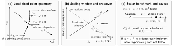
A fixed point organizes local flow, not every global trajectory. Panel (a) shows the critical surface tangent to the irrelevant eigendirection and the relevant departure under infrared flow. Panel (b) compares $e^{\theta\ell}$ growth with $e^{-\omega\ell}$ corrections for $\ell=\ln(\Lambda/k)$. Panel (c) shows the tuned one-loop $O(N)$ scalar trajectory from the Gaussian point to $g_\star=6\epsilon/(N+8)$ and the dangerously irrelevant-coupling exception to naive hyperscaling. The diagram is schematic and not to scale.

When hyperscaling fails or changes form

The regularity assumption in the irrelevant arguments is the vulnerable step. Suppose

$$f_{\mathrm{s}}(\tau,h,u) =b^{-d} \mathcal F \left( b^{y_t}\tau, b^{y_h}h, b^{y_u}u \right), \qquad y_u<0,$$

but $\mathcal F$ is singular as its last argument tends to zero. Then $u$ is dangerously irrelevant. The powers extracted by simply dropping $u$ need not describe the observable.

Above four dimensions, the scalar quartic coupling supplies the standard check. The Gaussian fixed point gives $y_u=4-d<0$, but the ordered-phase Landau minimum has $M^2=-r/u$ and $f_{\min}=-r^2/(4u)$. The $u^{-1}$ singularity invalidates $f_{\mathrm s}\sim\xi^{-d}$. Mean-field values $\alpha=0$ and $\nu=1/2$ would imply

$$2-\alpha=2, \qquad d\nu=\frac d2,$$

which disagree for $d>4$. Rushbrooke, Widom, and Fisher relations can still hold while Josephson hyperscaling fails. At the upper critical dimension $d=4$, the leading powers happen to satisfy $2-\alpha=d\nu$, but the marginal quartic produces multiplicative logarithms, so a pure-power ansatz is incomplete. Fisher gives the dangerous-variable analysis in Fisher 1983, §§ 4–5, pp. 35–55.

Other modifications require their own declared scaling structure: anisotropic fixed points can have several correlation-length exponents; boundaries have surface exponents; long-range interactions change the field dimension; and systems with a hyperscaling-violation exponent $\vartheta$ use an effective free-energy dimension $d-\vartheta$. None should be diagnosed merely because a finite-window fit misses one equality.

Fixed-point evidence matrix

An exponent estimate inherits the assumptions of the method that produced it. The table separates five evidence routes by their inputs, direct outputs, dominant systematics, and claim ceiling. Read each row horizontally: agreement across rows is valuable because the limitations are different, not because every route measures exactly the same object.

Evidence route	Essential assumptions and control	Direct outputs or observables	Dominant systematics and evidence ceiling
Perturbative expansion	A small $\epsilon$, weak fixed-point coupling, large-$N$ parameter, or other declared expansion; specified renormalization scheme and operator sector	Beta-function zeros, stability eigenvalues, anomalous dimensions, and resummed exponent or amplitude-ratio estimates	Missing orders, asymptotic-series resummation, scheme and operator truncation; controlled local evidence within the expansion domain, not a global existence proof at order-one parameters
Lattice finite-size scaling	A Euclidean discretization in the target basin; controlled critical, continuum, and infinite-volume limits; reflection positivity when used	Correlation lengths, step scaling, Binder-type ratios, spectra, exponents, amplitude ratios, and scaling functions	Cutoff and volume extrapolation, critical tuning, autocorrelation, action dependence, and analytic continuation; strong nonperturbative IR evidence for the simulated universality class
Functional RG	An exact flow equation combined with a declared ansatz, projection, regulator, identity constraints, and convergence tests	Global flow portraits, effective potentials, fixed-point spectra, equations of state, and crossover trajectories	Truncation, projection, regulator dependence, symmetry identities, convexity, and numerics; quantitative candidate evidence unless convergence is independently controlled
Conformal bootstrap	Conformal invariance, crossing, a symmetry sector, unitarity or reflection positivity when imposed, and explicit gap assumptions	Allowed or excluded regions for operator dimensions and OPE coefficients; islands and universal CFT data	Derivative and spin truncations, assumed gaps, navigator or optimization choices, and numerical certification; characterizes or excludes a CFT under stated assumptions but does not supply an RG trajectory
Rigorous or constructive analysis	A precise lattice or continuum model, norm, positivity domain, and theorem hypotheses, often in restricted dimensions or coupling ranges	Existence or nonexistence, controlled continuum correlations, bounds, and in some cases complete RG trajectories	Transfer is limited by theorem hypotheses and model class; strongest conclusion inside the proved domain, with no automatic extension to nearby physical theories

Representative primary analyses illustrate the distinct ceilings: the epsilon expansion constructs a perturbative fixed point Wilson and Fisher 1972, pp. 240–243; finite-size lattice scaling controls volume and correction terms Hasenbusch 2010, §§ II–V; effective-average-action studies expose truncation and regulator choices Berges, Tetradis, and Wetterich 2002, §§ 2–3, pp. 245–287; bootstrap bounds assume crossing and unitarity El-Showk et al. 2012, §§ II–IV; and rigorous construction can establish a complete trajectory for a precisely defined modified model Abdesselam 2007, pp. 727–772.

The matrix is not a ranking. A theorem about a restricted model, a high-order perturbative series, a converged lattice result, a stable functional truncation, and a bootstrap island answer different questions. A strong universality claim identifies which assumptions overlap and which conclusions are genuinely independent.

Critical Surfaces, Crossover, and Corrections to Scaling next turns the relevant and irrelevant exponents into tuning conditions and departure scales.

Common pitfalls

Treating derived exponents as independent measurements. If $\beta_{\mathrm{mag}}$, $\gamma$, and $\delta$ were computed from the same $\nu$ and $\eta$ using scaling relations, their agreement with those relations is an algebraic check, not three independent confirmations.

Using hyperscaling without testing irrelevant variables. The sign $y_u<0$ only says that $u$ flows to zero. One must also check that the observable’s scaling function is regular there.

Mixing asymptotic orders. Scaling relations must be tested after every expression is expanded to a common perturbative order. Unexpanded ratios can contain uncontrolled higher-order terms.

Fitting outside the scaling window. Far from criticality, analytic backgrounds and crossover dominate; too close in a finite system, finite-size rounding dominates. A stable result varies both ends of the fit window and includes justified correction terms.

Exercises

1. Reconstruct the exponent set

In $d=3$, take $\nu=0.64$ and $\eta=0.05$. Assuming ordinary hyperscaling, compute $y_t$, $y_h$, $\alpha$, $\beta_{\mathrm{mag}}$, $\gamma$, and $\delta$.

Solution

The two RG eigenvalues are

$$y_t=\nu^{-1}=1.5625, \qquad y_h=\frac{3+2-0.05}{2}=2.475.$$

Then

$$\begin{aligned} \alpha&=2-3(0.64)=0.08,\\ \beta_{\mathrm{mag}}&=0.64(3-2.475)=0.336,\\ \gamma&=0.64(1.95)=1.248,\\ \delta&=\frac{2.475}{0.525}=\frac{33}{7}\simeq4.714. \end{aligned}$$

The rounded values satisfy $\alpha+2\beta_{\mathrm{mag}}+\gamma=2$.

2. Translate the leading correction

An observable has $\nu=0.70$ and a leading irrelevant exponent $\theta_{\mathrm{irr}}=-0.90$. What correction powers appear in a finite-size fit at criticality and in a reduced-temperature fit in infinite volume?

Solution

The correction exponent is $\omega=0.90$. At criticality the finite-size correction is proportional to $L^{-0.90}$. In an infinite-volume fit versus $\tau$, it is proportional to $|\tau|^{\omega\nu}=|\tau|^{0.63}$. Their amplitudes need not be the same.

3. Locate the failed assumption above four dimensions

Use the mean-field values $\alpha=0$, $\beta_{\mathrm{mag}}=1/2$, $\gamma=1$, $\delta=3$, $\nu=1/2$, and $\eta=0$ in $d=5$. Test all four displayed scaling relations.

Solution

Rushbrooke gives $0+2(1/2)+1=2$, Widom gives $1=(1/2)(3-1)$, and Fisher gives $1=(1/2)(2-0)$. All three hold. Josephson hyperscaling gives $2-0=2$ on the left but $5(1/2)=2.5$ on the right, so it fails. The dangerous quartic invalidates the free-energy-per-correlation-volume assumption, not the other three algebraic statements.

4. Identify independent evidence

A functional-RG calculation reports $\nu$ and derives $\alpha$ from hyperscaling. A lattice study measures $\nu$ from a correlation-length crossing and measures the singular free-energy exponent independently. Which comparison tests hyperscaling?

Solution

The functional-RG pair does not independently test hyperscaling because $\alpha$ was defined from $2-d\nu$. The lattice comparison can test it if the continuum, volume, tuning, and background systematics of the two measurements are controlled and their covariance is included. Agreement between the FRG value of $\nu$ and the lattice value is a separate cross-method check.

References

• Abdesselam, Abdelmalek. “A Complete Renormalization Group Trajectory Between Two Fixed Points.” Communications in Mathematical Physics 276 (2007): 727–772. DOI. Open PDF.
• Berges, Jürgen, Nikolaos Tetradis, and Christof Wetterich. “Non-Perturbative Renormalization Flow in Quantum Field Theory and Statistical Physics.” Physics Reports 363 (2002): 223–386. DOI. Open PDF.
• El-Showk, Sheer, Miguel F. Paulos, David Poland, Slava Rychkov, David Simmons-Duffin, and Alessandro Vichi. “Solving the 3D Ising Model with the Conformal Bootstrap.” Physical Review D 86 (2012): 025022. DOI. Open PDF.
• Fisher, Michael E. “Scaling, Universality and Renormalization Group Theory.” In Critical Phenomena, Lecture Notes in Physics 186, 1–139. Berlin: Springer, 1983. DOI.
• Fisher, Michael E. “The Theory of Equilibrium Critical Phenomena.” Reports on Progress in Physics 30 (1967): 615–730. DOI.
• Hasenbusch, Martin. “Finite Size Scaling Study of Lattice Models in the Three-Dimensional Ising Universality Class.” Physical Review B 82 (2010): 174433. DOI. Open PDF.
• Wegner, Franz J. “Corrections to Scaling Laws.” Physical Review B 5 (1972): 4529–4536. DOI.
• Wilson, Kenneth G., and Michael E. Fisher. “Critical Exponents in 3.99 Dimensions.” Physical Review Letters 28 (1972): 240–243. DOI.