

Soft-Collinear Effective Theory: Architecture and Validity
Soft-collinear effective theory is a family of gauge theories for processes with energetic particles confined to narrow lightlike directions and lower-momentum radiation. Hard fluctuations are encoded in Wilson coefficients; each energetic direction becomes a collinear sector; long-wavelength fields are multipole expanded; and gauge invariance packages unresolved emissions into Wilson lines. The hierarchy and measurement select the modes—there is no universal SCET field list.
This page assembles the named architecture. It constructs the leading-power two-jet current using label and residual momenta, sector gauge symmetries, collinear building blocks, and soft Wilson lines. The general proofs of multipole expansion, factorization, and evolution remain on the preceding method pages; here they become validity conditions for choosing an SCET variant.
Required background. Modes, Virtualities, and EFT Scale Separation supplies the mode-selection tests. Matching onto Factorized Operator Structures supplies the conditions under which a sector current becomes an observable factorization theorem. Evolution Kernels, Consistency Relations, and Resummation Architecture supplies the RG construction.
Helpful background. Running and Matching across Multiple Thresholds clarifies staged matching. Mellin Transforms and Scaling Asymptotics is useful when convolutions become products in moment space.
SCET is selected by a hierarchy and measurement
Section titled “SCET is selected by a hierarchy and measurement”Choose null reference vectors for the energetic directions. For a two-jet problem, let , , and order components as . A standard SCET hierarchy is
The collinear virtuality is , while the ultrasoft virtuality is . At leading power the baseline action has the form
Before soft decoupling, contains the multipole-expanded eikonal coupling to the ultrasoft background. Different collinear directions do not couple through ordinary local vertices; hard interactions that change directions reside in external operators. Glauber potentials, when leading, are additional operators rather than part of this baseline sum.
The common variants are distinguished by physical scaling, not only by names:
| Architecture | Long-wavelength scaling | Virtuality relation | Additional requirement | Typical use |
|---|---|---|---|---|
| SCET | Ultrasoft | Ordinary virtuality evolution and overlap subtraction | Two-jet thrust and endpoint spectra | |
| SCET | Soft-II | but rapidities differ | Rapidity regulator, evolution, and compatible zero-bins | Small transverse momentum and broadening-type observables |
| SCET | Collinear-soft or soft-collinear modes fixed by an extra hierarchy | Intermediate virtuality or rapidity scales | Additional matching stage and nested overlaps | Nearby jets, soft jets, or several resolution scales |
| Glauber-extended SCET | Transverse-potential scaling selected by a pinch | Observable dependent | Explicit Glauber operators, causal prescriptions, and cut analysis | Forward or spectator-sensitive hadronic scattering |
For example, resolving two nearby jets introduces a collinear-soft mode that is soft relative to either daughter jet but collinear relative to their parent direction. Pietrulewicz, Tackmann, and Waalewijn construct these modes and the matching back to ordinary SCET when the extra hierarchy disappears in Pietrulewicz, Tackmann, and Waalewijn 2016, §§ 1–2.6, preprint pp. 1–16, Open PDF.
Label fields and the leading action
Section titled “Label fields and the leading action”In the label-momentum formulation of SCET, split an -collinear momentum into
The large and transverse components are labels; derivatives on the residual field return . Thus
and the label operator satisfies
Only the sum is physical. Small shifts between label and residual momentum leave predictions unchanged, and changes of and that preserve their null normalization are constrained by reparameterization invariance. These redundancies restore the Lorentz information hidden by the light-cone decomposition.
The large collinear spinor is
With , its leading Lagrangian is
where
The inverse derivative is nonlocal along the large light-cone direction and becomes a collinear Wilson line. The remaining field scalings are
They make every term in the leading action homogeneous. Bauer, Fleming, Pirjol, and Stewart derive the label split, field scaling, collinear action, and gauge-invariant completion in Bauer et al. 2001, §§ II–III and Appendix A, pp. 4–16 and 30–32, Open PDF.
Sector gauge symmetry and Wilson-line building blocks
Section titled “Sector gauge symmetry and Wilson-line building blocks”An -collinear gauge transformation carries -collinear Fourier support and acts only on that sector; a long-wavelength transformation acts as a slowly varying background color rotation evaluated at the multipole point. Separate transformations exist for every collinear direction. Their consequences are summarized by
| Symmetry | Acts on | Required completion |
|---|---|---|
| -collinear quarks and gluons | , , and | |
| -collinear quarks and gluons | , , and | |
| Ultrasoft fields and each collinear sector at its projected coordinate | Wilson lines after soft decoupling | |
| Reparameterization invariance | Reference directions and label/residual split | Relations among operators and Wilson coefficients |
For a line extending to past infinity, define
If , then . The combinations
are invariant under ; brackets mean that the derivative acts only inside them. A hard-scattering basis is built from these blocks, label operators, and color tensors rather than from bare collinear fields.
At leading power, ultrasoft gluons couple eikonally through . Introduce
where and the associated prescription distinguish incoming from outgoing lines. The field redefinition
removes ultrasoft fields from the leading collinear Lagrangian but moves into hard operators. Bauer, Pirjol, and Stewart derive the separate gauge symmetries and this leading-power decoupling in Bauer, Pirjol, and Stewart 2002, §§ III–IV, pp. 4–18, Open PDF.
First application: construct the leading dijet current
Section titled “First application: construct the leading dijet current”Match the color-singlet QCD current at timelike momentum transfer onto one -collinear and one -collinear building block. Define label-projected fields by
where denote the large momentum magnitudes; field-flow conventions determine the corresponding signed labels. The complete leading vector structure is
For back-to-back massless kinematics, . The construction passes four immediate checks:
- before label projection, has mass dimension three and scales as ; the conventional label measure preserves the current dimension;
- each is invariant under its own collinear gauge group, so no bare sector field remains;
- the projected spinors leave a transverse vector structure, with at leading power; and
- reparameterization invariance makes the coefficient depend on the hard invariant , not on an arbitrary normalization of or .
At tree level . Loop matching subtracts the EFT infrared matrix element from the renormalized QCD form factor and leaves an infrared-finite coefficient.
After the soft-decoupling redefinition, the same current becomes
This is the leading SCET dijet architecture: a hard coefficient, two separately collinear-gauge-invariant fields, and a causal soft Wilson-line product. It is not yet a cross-section theorem. The measurement operator must separate at leading power, overlaps must be subtracted, and Glauber exchange must cancel or be retained explicitly before matrix elements may be called independent hard, jet, and soft functions.
Choosing a variant and recognizing its limits
Section titled “Choosing a variant and recognizing its limits”Use the following sequence before applying a standard SCET formula:
| Question | If yes | If no or unresolved |
|---|---|---|
| Are energetic directions separated by hard invariants while each jet mass is parametrically smaller? | Introduce one collinear sector per resolved direction | SCET is unnecessary or the directions require a parent sector and later matching |
| Do collinear and long-wavelength modes have different virtualities? | Use an SCET-type virtuality sequence | If virtualities coincide but rapidities differ, use SCET and two-scale evolution |
| Does the observable resolve another energy, angle, radius, or veto hierarchy? | Test collinear-soft or soft-collinear modes and staged matching | Do not force all logarithms into the ordinary hard–jet–soft factors |
| Is every leading overlap defined and subtracted in the chosen regulator? | Proceed to renormalization checks | Stop: a sector sum with double counting has no physical interpretation |
| Does the measurement separate after multipole expansion? | Construct measured sector matrix elements | Keep a coupled measurement operator or use a more general multiplicity-space factorization |
| Are endpoint convolutions finite as renormalized distributions? | Use the ordinary kernel architecture | Refactorize the endpoint or add the mode/operator required by the limiting region |
| Are Glauber pinches absent, canceled, or represented by operators? | State the proven condition | Restrict the claim and use the Glauber-factorization analysis |
Non-global measurements require their own color- and multiplicity-space evolution rather than an automatic four-function product; the observable definition and non-global caution belong with Jets and Event-Shape Observables. Nonperturbative soft or collinear scales require operator matrix elements or shape functions and limit purely perturbative predictions.
Stable core and current research boundary
Section titled “Stable core and current research boundary”Evidence status, checked through 3 August 2026. The leading-power dijet construction above is mature. Its representation and extensions remain more delicate than a fixed list of fields suggests.
First, labels and an explicit ultrasoft field are not the invariant essence of the theory. Goerke and Luke formulate the two-sector problem as decoupled copies of QCD coupled by Wilson lines, without an explicit ultrasoft field at the hard matching scale, and recover the same infrared physics when sector overlaps are subtracted correctly. This provides a useful contrary formulation and makes boost invariance manifest; it does not remove the need to account for the overlap. See Goerke and Luke 2018, §§ 1–3, preprint pp. 1–16, Open PDF.
Second, leading-power BPS decoupling cannot simply be copied to every power correction. At order , position-space soft-quark–hard-collinear interactions can produce off-shell radiative jet functions that are not separately gauge invariant until equation-of-motion terms restore the missing contributions. The S-matrix remains gauge invariant, but an ostensibly invariant subleading building block need not define a valid factor by itself. See Bodwin et al. 2024, abstract and §§ I, V–IX, pp. 1–3 and 19–28, Open PDF.
Third, “Glauber exchange breaks factorization” is too broad. For gap-between-jets production, Becher and collaborators identify perturbative active–active Glauber contributions whose three-loop structure converts the problematic double-logarithmic low-scale evolution into the form required by PDF factorization. They explicitly stop short of an all-order proof. The lesson is to include and test the relevant region, not to assume either cancellation or violation. See Becher et al. 2025, pp. 1–5, Open PDF.
The SCET architecture in the mode map
Section titled “The SCET architecture in the mode map”The left panel separates the SCET ultrasoft point from collinear modes by virtuality and places the SCET soft point on the equal-virtuality rapidity line. The right panel is the construction order used on this page: select modes, promote them to homogeneous fields, expand and subtract overlaps, match gauge-invariant sector operators, and only then evolve and test factorization.
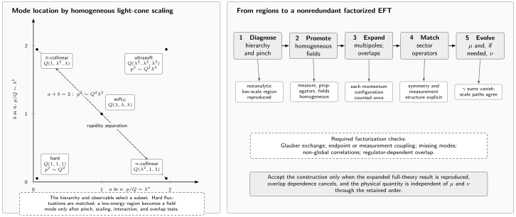
Mode locations are shown in the exponents and of , with the transverse exponent written in each label. The line contains -collinear, -collinear, and soft-II scalings of virtuality ; their separation along the line is a rapidity separation. Ultrasoft momentum has virtuality , while hard fluctuations are matched at . The points are alternatives selected by a hierarchy and observable, not a universal simultaneous field list. A consistent construction requires homogeneous fields, multipole and overlap expansion, sector matching, and and, when needed, evolution, with explicit factorization checks. The diagram is schematic and not to scale.
Common pitfalls
Section titled “Common pitfalls”Treating SCET and SCET as interchangeable notation. Their long-wavelength virtualities differ. Equal-virtuality sectors need rapidity renormalization that is absent from the simplest SCET treatment.
Giving labels physical significance. The label–residual split and the normalization of are redundant. Only total momenta, invariant matching variables, and reparameterization-invariant operator combinations may enter a prediction.
Calling Wilson-line dressing a factorization proof. establishes collinear gauge invariance and organizes leading eikonal interactions. Measurements, overlaps, endpoints, and Glauber exchange remain independent conditions.
Extending leading-power decoupling without a new analysis. Subleading Lagrangian insertions reconnect sectors and can require new radiative functions, equation-of-motion terms, and renormalization kernels.
Exercises
Section titled “Exercises”-
What information belongs to the hard current coefficient rather than to jet functions?
Solution
contains physics of virtuality of order and the corresponding hard logarithms. Collinear infrared poles, small invariant masses, and measurement dependence belong to the collinear and soft matrix elements.
-
Why does the leading soft-field redefinition not remove soft physics from the process?
Solution
It moves leading soft interactions from the collinear Lagrangian into Wilson lines in external operators. Their matrix elements remain as the soft function and continue to carry the process’s long-distance eikonal physics.
References
Section titled “References”-
Bauer, Christian W., Sean Fleming, Dan Pirjol, and Iain W. Stewart. 2001. “An Effective Field Theory for Collinear and Soft Gluons: Heavy to Light Decays.” Physical Review D 63 (11): 114020. DOI. Open PDF.
-
Bauer, Christian W., Dan Pirjol, and Iain W. Stewart. 2002. “Soft-Collinear Factorization in Effective Field Theory.” Physical Review D 65 (5): 054022. DOI. Open PDF.
-
Becher, Thomas, Patrick Hager, Sebastian Jaskiewicz, Matthias Neubert, and Dominik Schwienbacher. 2025. “Factorization Restoration through Glauber Gluons.” Physical Review Letters 134 (6): 061901. DOI. Open PDF.
-
Bodwin, Geoffrey T., June-Haak Ee, Daekyoung Kang, and Xiang-Peng Wang. 2024. “Gauge Invariance of Radiative Jet Functions in the Position-Space Formulation of SCET.” Physical Review D 109 (5): 056020. DOI. Open PDF.
-
Goerke, Raymond, and Michael Luke. 2018. “Power Counting and Modes in SCET.” Journal of High Energy Physics 2018 (2): 147. DOI. Open PDF.
-
Pietrulewicz, Piotr, Frank J. Tackmann, and Wouter J. Waalewijn. 2016. “Factorization and Resummation for Generic Hierarchies between Jets.” Journal of High Energy Physics 2016 (8): 002. DOI. Open PDF.
Original QFT.org content:CC BY 4.0, unless an item supplies different terms. Third-party material retains its own terms.