Hierarchies, Thresholds, and Fine-Tuning Measures

A fine-tuning measure summarizes a cancellation or a local response inside a declared parameterization. It can reveal that a low-energy quantity changes rapidly when selected high-scale inputs are varied independently, but it is not itself an observable and it does not define a probability without a normalized measure and conditioning rule.

This page evaluates two common diagnostics for the light scalar and heavy threshold introduced previously. The calculation makes coordinate choice, correlations, matching scale, and prior dependence explicit; it does not rank current models.

Required background. Scale Sensitivity and Radiative Stability derives the matched scalar-mass relation used here.

Helpful background. Probability Spaces, Random Variables, and Conditional Expectation supplies the measure-theoretic distinction between a diagnostic and a probability. Running and Matching across Multiple Thresholds supplies the staged evolution needed when more than one heavy scale is present.

One hierarchy supports several diagnostics

At the matching scale $\mu=M$, the one-loop relation for the two-scalar model is

$$O\equiv m_<^2 = a+b, \qquad a\equiv m_>^2, \qquad b\equiv-\frac{\lambda M^2}{32\pi^2}.$$

The quantities $a$ and $b$ are not separately observable; they are terms in a specified $\overline{\mathrm{MS}}$ matching decomposition. The pole mass obtained after light-field self-energy corrections is observable. Keeping that distinction visible prevents a convenient decomposition from being mistaken for a unique physical partition.

A correction-to-result ratio is

$$R_{\mathrm{th}} = \frac{|b|}{|O|}.$$

A symmetric cancellation diagnostic is

$$C = \frac{|a|+|b|}{|a+b|}.$$

Both become large when individually large terms leave a small remainder, but their normalizations differ. Neither asks how the remainder responds to a change of coordinates.

The Barbieri–Giudice local-sensitivity measure instead begins with independent inputs $x_i$ and a chosen output $O$:

$$\Delta_{x_i} = \left| \frac{\partial\ln |O|}{\partial\ln |x_i|} \right|, \qquad \Delta_{\mathrm{BG}} = \max_i\Delta_{x_i}.$$

This logarithmic derivative was introduced as a model-parameter sensitivity criterion by Barbieri and Giudice 1988, § 2, pp. 65–67. It is local, differential, and conditional on the input chart and scale.

If $a$ and $M^2$ are independent while $\lambda$ is fixed, then

$$\Delta_a = \left|\frac{a}{O}\right|, \qquad \Delta_{M^2} = \left|\frac{b}{O}\right|, \qquad \Delta_{\mathrm{BG}} = \max\!\left( \frac{|a|}{|O|}, \frac{|b|}{|O|} \right).$$

Using $M$ rather than $M^2$ doubles the second logarithmic derivative:

$$\Delta_M=2\Delta_{M^2}.$$

That factor is not a loop ambiguity. It is the Jacobian between two parameter coordinates.

A numerical comparison

Take

$$M=10~\mathrm{TeV}, \qquad \lambda=0.1, \qquad O=(0.1~\mathrm{TeV})^2.$$

The threshold and required parent mass are

$$\begin{aligned} b&=-0.0316629~\mathrm{TeV}^2,\\ a&=O-b=0.0416629~\mathrm{TeV}^2. \end{aligned}$$

The two diagnostics give

$$R_{\mathrm{th}}=3.166, \qquad C=7.333, \qquad \Delta_{\mathrm{BG}}(a,M^2)=4.166.$$

If the input chart uses $(a,M)$, the heavy-scale component becomes $6.333$, so the maximum becomes $6.333$. All numbers describe the same matched relation. Their disagreement is useful: it identifies which convention each diagnostic encodes.

A report should therefore quote the vector $(\Delta_{x_1},\ldots,\Delta_{x_n})$ before collapsing it to a maximum, norm, percentile, or threshold. The reduction discards direction and correlation information.

Reparameterization changes a local sensitivity

Let one positive input be replaced by

$$y=\left(\frac{x}{x_0}\right)^n, \qquad n\ne0.$$

The chain rule gives

$$\frac{\partial\ln|O|}{\partial\ln y} = \frac{1}{n} \frac{\partial\ln|O|}{\partial\ln x}.$$

An arbitrary choice of $n$ rescales the sensitivity. This proves that a bare logarithmic derivative is not a scalar on parameter space. It remains a legitimate diagnostic once the physically independent coordinates have been motivated—for example, Wilson coefficients at a specified matching scale—but the motivation is part of the result.

The same issue appears under a finite scheme transformation. A redefinition

$$a'=a+\kappa b, \qquad b'=(1-\kappa)b$$

leaves $O=a'+b'=a+b$ unchanged but reallocates the apparent cancellation. Calculated observables agree after consistent conversion; contribution-wise measures need not. Scheme variation is therefore a robustness check, not a search for a uniquely “true” split.

Correlated inputs define a different derivative

Suppose a parent theory constrains

$$a(M^2)=a_0+\rho M^2.$$

Along that allowed one-dimensional surface,

$$\frac{dO}{dM^2} = \rho-\frac{\lambda}{32\pi^2},$$

whereas the partial derivative at fixed $a$ is $-\lambda/(32\pi^2)$. If $\rho$ is close to the threshold coefficient, the total derivative focuses even though the two terms in a particular coordinate split are individually large. If the relation is not enforced by the parent theory, imposing it merely hides an independent variation.

RG focusing is the scale-dependent version of this statement. Let high-scale inputs $x_i(\Lambda)$ evolve to $O(\mu)$. The relevant derivative is the composite map

$$\frac{\partial O(\mu)}{\partial x_i(\Lambda)} = \frac{\partial O}{\partial c_A(\mu)} \frac{\partial c_A(\mu)}{\partial x_i(\Lambda)},$$

including every matching matrix between $\Lambda$ and $\mu$. A focus point is meaningful only with the boundary scale, independent inputs, thresholds, and perturbative accuracy stated. The sensitivity can move when any of these change.

A probability requires a prior and likelihood

The figure locates tuning diagnostics in the conditional branch, separate from both calculated thresholds and probabilities. Inspect the right-hand boxes: parameter coordinates select derivative components, while a prior supplies an additional measure. Neither is fixed by the loop calculation.

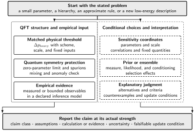
A calculated threshold, a coordinate-dependent sensitivity, and a probability distribution are distinct objects. The first follows from matching, the second from a selected parameter chart and variation rule, and the third additionally requires a normalized measure and conditioning data. The diagram is schematic and not to scale.

For parameters $x$ with prior density $\pi(x)$ and data $D$ with likelihood $L(D\mid x)$, a probability for a hierarchy region $H$ is

$$P(H\mid D) = \frac{ \displaystyle\int_H dx\,\pi(x)L(D\mid x) }{ \displaystyle\int dx\,\pi(x)L(D\mid x) }.$$

Under a one-to-one change $y=f(x)$, the same probability is preserved only if

$$\pi_y(y) = \pi_x(x(y)) \left|\frac{dx}{dy}\right|.$$

Declaring a density flat in both $x$ and nonlinear $y$ does not perform the same inference; it changes the prior. Jeffreys’s invariant-prior construction is one response for regular statistical models, but it still depends on the likelihood and model family Jeffreys 1946, pp. 453–461.

A simple cancellation illustrates the distinction. Fix $b<0$, take $a$ uniformly distributed on $[-A,A]$, and assume $|b|+\delta<A$. Then

$$P(|a+b|<\delta) = \frac{2\delta}{2A} = \frac{\delta}{A}.$$

A log-uniform prior on positive $a$, conditioned to a finite interval, gives a different probability near $a=|b|$. Neither follows from $R_{\mathrm{th}}$ alone. Prior normalization, range, correlations, likelihood, and selection effects must be reported before “one part in $N$” is a probability statement. Anderson and Castaño’s proposal to compare sensitivity with a parameter-space average already makes this dependence on a chosen domain explicit Anderson and Castaño 1995, pp. 300–304.

Claim-classification table

The table keeps the matched correction, sensitivity diagnostic, and probabilistic typicality in separate rows. A strong analysis may use all three, but it must not substitute one for another.

Claim class	Evidence or mathematical object	Conditional choices that must be declared	Licensed conclusion	Does not establish
Calculated threshold	Renormalized parent-to-EFT matching relation	Scheme, matching scale, matched observable, fixed inputs, and perturbative order	Size and operator structure of a heavy-scale contribution in that relation	Probability, inconsistency, or a preferred UV theory
Technical stability	Enhanced quantum symmetry, Ward identities, and spurion selection rules	Field content, symmetry limit, anomaly status, thresholds, basis, and retained order	Which corrections vanish or carry declared symmetry-breaking factors	Numerical value, typicality, or empirical success
Sensitivity diagnostic	Cancellation ratio or derivative such as $\partial\ln O/\partial\ln a_i$	Parameter coordinates, correlations, scale, observable, and quantities held fixed	Local response or cancellation in the declared chart	Coordinate-free observable, probability, or universal model ranking
Probabilistic typicality	Normalized measure, prior, likelihood, and posterior	Sample space, measure, conditioning data, selection effects, and parameterization	Probability within the declared ensemble and inference model	Ensemble-independent fact or theorem of QFT
Empirical fact	Measurement, exclusion, or reproducible bound	Dataset, likelihood, model assumptions, date, and validity domain	What observations favor or exclude within those assumptions	A unique explanatory principle or prior
Explanatory heuristic	Comparative argument about autonomy, simplicity, mechanism, or research priority	Alternatives, virtues, counterexamples, historical scope, and update conditions	A transparent conditional preference or strategy	Calculation, symmetry theorem, probability, or empirical result

Reporting and robustness checks

A reproducible tuning claim states:

1. the observable or renormalized output and whether it is an input or prediction;
2. the parent theory, EFT, scheme, matching scales, and perturbative order;
3. the independent parameter chart and any exact or statistical correlations;
4. the derivative direction, finite variation, cancellation norm, or other functional;
5. the high and low scales connected by matching and RG evolution;
6. the prior, range, likelihood, data, and selection rule if probability language is used;
7. the result under at least one physically motivated reparameterization or scheme conversion; and
8. the omitted-order uncertainty and update condition.

Useful stress tests recompute the result with $M$ versus $M^2$, expose component sensitivities before taking a maximum, propagate the UV covariance matrix, vary matching scales, and compare nearby schemes at the same perturbative order. Large changes do not invalidate the underlying threshold calculation; they delimit what the chosen diagnostic can support. Wider discussions of these distinctions and their historical use appear in Giudice 2008, §§ 2–4, pp. 5–17, Open PDF and Craig 2022, §§ 1–2 and 5, pp. 1–7 and 18–21, Open PDF.

Common pitfalls

Calling a maximum derivative an observable. $\Delta_{\mathrm{BG}}$ depends on coordinates, scale, and the independent-input declaration. Report those choices with the number.

Using a partial derivative across a constrained surface. If a parent theory correlates parameters, differentiate along that surface. If no mechanism enforces the correlation, do not add it merely to reduce sensitivity.

Changing coordinates while silently resetting the prior. The Jacobian-transformed density represents the same measure. A newly flat density represents a different inference problem.

Ignoring thresholds between input and output scales. A high-scale derivative must pass through each matching and running map. Omitting one can create or erase apparent focusing.

Reporting more precision than the EFT calculation. Sensitivities built from cancellations can amplify truncation errors. Propagate matching, running, and input uncertainty before quoting significant digits.

References

• Anderson, Gordon W., and Diego J. Castaño. 1995. “Measures of Fine Tuning.” Physics Letters B 347: 300–308. DOI.

• Barbieri, Riccardo, and Gian F. Giudice. 1988. “Upper Bounds on Supersymmetric Particle Masses.” Nuclear Physics B 306: 63–76. DOI.

• Craig, Nathaniel. 2022. “Naturalness: A Snowmass White Paper.” arXiv:2205.05708 [hep-ph]. arXiv. Open PDF.

• Giudice, Gian Francesco. 2008. “Naturally Speaking: The Naturalness Criterion and Physics at the LHC.” In Perspectives on LHC Physics, edited by G. Kane and A. Pierce, 155–178. World Scientific. DOI. Open PDF.

• Jeffreys, Harold. 1946. “An Invariant Form for the Prior Probability in Estimation Problems.” Proceedings of the Royal Society A 186: 453–461. DOI.