Regulator Removal and Renormalized Predictions

A regulated calculation becomes a renormalized prediction only after three operations are kept distinct: finite inputs are fixed, the regulator is removed or its residual artifacts are controlled, and a quantity not used as an input is shown to be stable. Bare parameters are allowed—and generally required—to vary along the removal trajectory. Holding them fixed usually changes the theory.

The evidence is stronger than cancellation of a symbol such as $\ln\Lambda$ or $1/\epsilon$. One must also verify locality of the subtractions, the relevant symmetry identities, dimensional consistency, the finite scheme map, and the expected order of both regulator artifacts and perturbative truncation. This page assembles those checks into Chapter 1’s exit test.

Required background. Renormalization Conditions, Schemes, and Finite Parts supplies the finite input conditions and MS̄-to-MOM map used below.

Helpful background. Interacting Fields, Asymptotic Observables, and Effective Descriptions distinguishes perturbative amplitudes, effective descriptions, and stronger existence claims.

A removal limit is taken at fixed renormalized inputs

Let $\rho$ denote regulator data: $\rho=\Lambda^{-1}$ for a momentum cutoff, $\rho=\epsilon$ for dimensional continuation, or another parameter appropriate to the definition. Choose $N$ independent finite inputs $\mathcal I_a^{\rm in}$ and solve

$$\mathcal I_a \bigl( p_0(\rho),\rho \bigr) = \mathcal I_a^{\rm in}, \qquad a=1,\ldots,N,$$

for the bare trajectory $p_0(\rho)$. A non-input quantity is then

$$\mathcal P_\rho(Q) = \mathcal P \bigl( Q;p_0(\rho),\rho \bigr).$$

The perturbative continuum criterion is

$$\lim_{\rho\to0} \mathcal P_\rho^{(L)}(Q) = \mathcal P_{\rm R}^{(L)}(Q)$$

at each retained loop order $L$, with the same limit obtained from other admissible regulators after matching the same inputs and restoring the same identities. The superscript is essential: an order-by-order perturbative limit is not automatically a nonperturbative construction of the theory.

The trajectory, rather than a fixed bare point, carries the finite theory through regulator space. Collins illustrates how bare couplings and field factors depend on a cutoff while renormalized quantities are held fixed Collins 1984/2023, § 7.10, p. 207, Eqs. (7.10.1)–(7.10.2).

Two regulators for the same scalar scattering prediction

Use the massive Euclidean $\mathbb Z_2$ scalar theory with $m>0$, fixed real Euclidean external momenta, and two finite inputs:

1. a mass fixed here by the Euclidean condition $\Gamma^{(2)}(0)=m^2$;
2. a four-point coupling $\lambda_*$ fixed at the symmetric point

$$P_s^2=P_t^2=P_u^2=Q_*^2>0.$$

The non-input quantity is the four-point coefficient at another set of channel momenta $P_s,P_t,P_u$. Define

$$F(P^2) \equiv \int_0^1dx\, \ln \frac{m^2+x(1-x)P^2}{\kappa^2},$$

where the arbitrary reference $\kappa$ cancels from the subtracted differences. All coupling expansions below are at a fixed regulator; the removal limit is taken on the subtracted coefficients, order by order.

Hard momentum cutoff

The one-loop tadpole is

$$\begin{aligned} A_\Lambda(m^2) &\equiv \int_{\lvert k\rvert<\Lambda} \frac{d^4k}{(2\pi)^4}\, \frac{1}{k^2+m^2} \\ &= \frac{1}{16\pi^2} \left[ \Lambda^2 -m^2\ln \left( 1+\frac{\Lambda^2}{m^2} \right) \right]. \end{aligned}$$

Imposing the Euclidean two-point input $\Gamma^{(2)}(0)=m^2$ gives

$$m_0^2(\Lambda) = m^2-\frac{\lambda_*}{2}A_\Lambda(m^2) +\mathcal O(\lambda_*^2).$$

The quadratically varying bare mass is required to keep the finite mass condition fixed. At this order the tadpole has no external-momentum dependence, so no field-strength trajectory is needed.

Use the unshifted sphere centered on the loop variable $k$:

$$B_\Lambda(P^2) \equiv \int_{\lvert k\rvert<\Lambda} \frac{d^4k}{(2\pi)^4}\, \frac{1}{(k^2+m^2)((k+P)^2+m^2)}.$$

The domain is part of this finite prescription: changing variables requires translating the domain too. Imposing a new centered sphere after a Feynman-parameter shift defines a different finite regulator. For the routing above, $c_{\rm cut}=-1$, and the large-$\Lambda$ form at fixed $m,P$ is

$$B_\Lambda(P^2) = \frac{1}{16\pi^2} \left[ \ln\frac{\Lambda^2}{\kappa^2} +c_{\rm cut} -F(P^2) \right] + \mathcal O \left( \frac{m^2+P^2}{\Lambda^2} \right).$$

The unrenormalized four-point coefficient is, through one loop,

$$\Gamma_\Lambda^{(4)} = \lambda_0(\Lambda) - \frac{\lambda_0^2(\Lambda)}{2} \sum_{X=s,t,u}B_\Lambda(P_X^2) +\mathcal O(\lambda_0^3).$$

Imposing $\Gamma_\Lambda^{(4)}|_{\rm sym}=\lambda_*$ at finite $\Lambda$ requires

$$\lambda_0(\Lambda) = \lambda_*+\frac{3\lambda_*^2}{2}B_\Lambda(Q_*^2) +\mathcal O(\lambda_*^3).$$

Its large-cutoff expansion is

$$\begin{aligned} \lambda_0(\Lambda) ={}& \lambda_* \\ &+ \frac{3\lambda_*^2}{32\pi^2} \left[ \ln\frac{\Lambda^2}{\kappa^2} +c_{\rm cut} -F(Q_*^2) \right] \\ &+ \mathcal O\left( \lambda_*^2\frac{m^2+Q_*^2}{\Lambda^2} \right) +\mathcal O(\lambda_*^3). \end{aligned}$$

At the displayed perturbative order, the bare coupling contains a cutoff logarithm. The exact finite-$\Lambda$ bubble in the first trajectory holds the MOM input fixed through the stated order; dropping its power corrections fixes that input only asymptotically.

Dimensional continuation

Set $d=4-2\epsilon$ and keep $\mu>0$ fixed. Define the continued loop integrals with a factor $\mu^{2\epsilon}$ in the loop measure:

$$\begin{aligned} A_\epsilon(m^2) &\equiv \mu^{2\epsilon} \int\frac{d^dk}{(2\pi)^d}\frac{1}{k^2+m^2} \\ &= \frac{\mu^{2\epsilon}}{(4\pi)^{2-\epsilon}} \Gamma(\epsilon-1)(m^2)^{1-\epsilon}, \\[4pt] B_\epsilon(P^2) &\equiv \mu^{2\epsilon} \int\frac{d^dk}{(2\pi)^d} \frac{1}{(k^2+m^2)((k+P)^2+m^2)} \\ &= \frac{\mu^{2\epsilon}}{(4\pi)^{2-\epsilon}} \Gamma(\epsilon) \int_0^1dx\, [m^2+x(1-x)P^2]^{-\epsilon}. \end{aligned}$$

The convergent starting domains are $1<\operatorname{Re}\epsilon<2$ for the tadpole and $0<\operatorname{Re}\epsilon<2$ for the massive bubble; the displayed gamma expressions then give their meromorphic continuations. In particular, $A_\epsilon$ has mass dimension two and $B_\epsilon$ is dimensionless. Schwinger parameters, the gamma-function continuation, and the explicit mass scale are developed in Collins 1984/2023, §§ 3.5–3.6.1, pp. 55–57. The formulas here are the Euclidean scalar loop integrals with their interaction and symmetry factors kept outside.

With $1/\bar\epsilon\equiv1/\epsilon-\gamma_E+\ln4\pi$, their expansions at fixed $m,\mu,P$ are

$$\begin{aligned} A_\epsilon(m^2) &= \frac{m^2}{16\pi^2} \left[ -\frac{1}{\bar\epsilon} +\ln\frac{m^2}{\mu^2} -1 \right] +\mathcal O(\epsilon m^2), \\ B_\epsilon(P^2) &= \frac{1}{16\pi^2} \left[ \frac{1}{\bar\epsilon} - \int_0^1dx\, \ln\frac{m^2+x(1-x)P^2}{\mu^2} \right] +\mathcal O(\epsilon). \end{aligned}$$

The identical two-point input requires

$$m_0^2(\epsilon) = m^2-\frac{\lambda_*}{2}A_\epsilon(m^2) +\mathcal O(\lambda_*^2),$$

using the exact continued $A_\epsilon$, including its terms beyond order $\epsilon^0$. Using only the displayed expansion would leave an additional $\mathcal O(\epsilon\lambda_*m^2)$ input error.

The bare coupling and proper four-point coefficient both have mass dimension $2\epsilon$. Set $\widetilde\lambda_0=\mu^{-2\epsilon}\lambda_0$. Their dimensionless one-loop relation is

$$\mu^{-2\epsilon}\Gamma_\epsilon^{(4)} = \widetilde\lambda_0 -\frac{\widetilde\lambda_0^2}{2} \sum_{X=s,t,u}B_\epsilon(P_X^2) +\mathcal O(\widetilde\lambda_0^3).$$

Thus the finite-dimensional MOM input is $\left.\mu^{-2\epsilon}\Gamma_\epsilon^{(4)}\right|_{\rm sym}=\lambda_*$. It fixes the exact continued bare trajectory through one loop:

$$\lambda_0(\epsilon) = \mu^{2\epsilon} \left\{ \lambda_*+\frac{3\lambda_*^2}{2}B_\epsilon(Q_*^2) +\mathcal O(\lambda_*^3) \right\}.$$

Expanding this trajectory near $\epsilon=0$ gives

$$\begin{aligned} \lambda_0(\epsilon) ={}& \mu^{2\epsilon} \bigg\{ \lambda_* \\ &+ \frac{3\lambda_*^2}{32\pi^2} \left[ \frac{1}{\bar\epsilon} - \int_0^1dx\, \ln \frac{m^2+x(1-x)Q_*^2}{\mu^2} \right] \\ &+ \mathcal O(\epsilon\lambda_*^2) +\mathcal O(\lambda_*^3) \bigg\}. \end{aligned}$$

The pole and the cutoff logarithm are not expected to resemble one another term by term. They are auxiliary local data in two different definitions. The common finite condition is the comparison point.

Common non-input result

Substitution of the exact finite-regulator trajectories gives, through one loop,

$$\Gamma_\rho^{(4),{\rm dimless}} = \lambda_*-\frac{\lambda_*^2}{2} \sum_{X=s,t,u} \left[B_\rho(P_X^2)-B_\rho(Q_*^2)\right] +\mathcal O(\lambda_*^3).$$

Here $\Gamma_\rho^{(4),{\rm dimless}}$ means $\Gamma_\Lambda^{(4)}$ for the cutoff and $\mu^{-2\epsilon}\Gamma_\epsilon^{(4)}$ for dimensional continuation. The bracket vanishes at the input for each regulator value. Removing the regulator at fixed inputs yields

$$\boxed{ \begin{aligned} \Gamma_{\rm R}^{(4)}(P;Q_*) ={}& \lambda_* \\ &+ \frac{\lambda_*^2}{32\pi^2} \left[ \sum_{X=s,t,u}F(P_X^2) -3F(Q_*^2) \right] \\ &+ \mathcal O(\lambda_*^3). \end{aligned} }$$

For the hard cutoff at finite $\Lambda$, append

$$\delta_{\rm reg}^{\Lambda} = \mathcal O \left[ \lambda_*^2 \frac{ m^2+\sum_XP_X^2+Q_*^2 }{\Lambda^2} \right],$$

This is a conservative bound for this scalar bubble and cutoff shape. The fixed-sphere calculation gives a sharper $\mathcal O(\Lambda^{-4})$ MOM remainder at fixed kinematics. For dimensional continuation before the final limit, append $\delta_{\rm reg}^{\epsilon}=\mathcal O(\epsilon\lambda_*^2)$. Both residuals vanish while the omitted perturbative contribution $\mathcal O(\lambda_*^3)$ remains.

After analytic continuation, the same channel logarithms and branch cuts appear in the scalar scattering amplitude. At this order the scalar field-strength correction vanishes, so no separate external residue changes the comparison. The cutoff and dimensional calculations therefore agree on a quantity not used to set $m$ or $\lambda_*$.

Residual artifacts and truncation are different errors

For a calculation through order $N$, compare regulated and continuum results at that same order:

$$\mathcal P_\rho^{[N]} = \mathcal P_{\rm cont}^{[N]} + \delta_{\rm reg}^{[N]}(\rho).$$

The regulator artifact $\delta_{\rm reg}^{[N]}$ is studied by changing $\rho$ at fixed renormalized inputs. It vanishes in the order-by-order removal limit. The omitted perturbative terms are a separate comparison: when an exact continuum prediction is defined for the same inputs and admits the stated asymptotic expansion, write

$$\mathcal P_{\rm exact} =\mathcal P_{\rm cont}^{[N]}+R_{\rm pert}^{[N+1]}, \qquad \mathcal P_\rho^{[N]}-\mathcal P_{\rm exact} =\delta_{\rm reg}^{[N]}(\rho)-R_{\rm pert}^{[N+1]}.$$

Thus removing the regulator does not remove the perturbative remainder. Higher-order calculations, power counting, scale dependence and calibrated diagnostics provide information about that remainder; an estimate of the first omitted order is not by itself a rigorous error bound for an asymptotic perturbation series.

For a cutoff calculation, use a fit form justified by the regulator and action, for example

$$\mathcal P_\Lambda = \mathcal P_\infty +\frac{a_1}{\Lambda^2} +\frac{a_2}{\Lambda^4} +\cdots$$

only when symmetry and large-$\Lambda$ expansion exclude lower powers or logarithmically modified powers. Fit several removal windows and test whether $\mathcal P_\infty$ is stable. Choose the powers from the actual subtracted observable and regulator; the bound above does not establish a leading $1/\Lambda^2$ law.

For dimensional continuation, a renormalized symbolic expression often permits the direct $\epsilon\to0$ limit. If numerical evaluation is used, test the expected expansion

$$\mathcal P_\epsilon = \mathcal P_0+b_1\epsilon+b_2\epsilon^2+\cdots$$

and increase numerical precision when poles cancel large intermediate terms. A flat plot at ordinary precision is not evidence if catastrophic cancellation hides the trend.

Scheme variation is a third diagnostic. After translating all inputs, a scheme difference should begin at the first omitted perturbative order; it should not scale like the regulator artifact. Keeping these signatures separate makes failures diagnosable.

Tests of the renormalized prediction

Calculations A and B are independent: dashed arrows impose the same finite inputs, while solid arrows bring their non-input outputs to the regulator-removal test. Compare the outputs at the same kinematics and order.

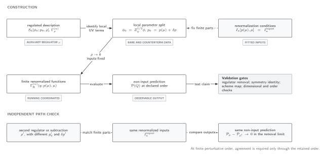
Each branch tunes its own bare parameters and allowed local counterterms before comparing $\mathcal P_A^{[N]}$ and $\mathcal P_B^{[N]}$. Here $\mathcal P$ is the fixed-normalization Euclidean four-point coefficient; continuation and external-state normalization give the scattering comparison described above. Vanishing regulator artifacts do not remove higher perturbative orders. This schematic map is not a proof of a nonperturbative continuum limit.

The common regulator-comparison fields extend to the following tests of a renormalized prediction:

Required field	What must be stated	Passing evidence
Regulated object	Action, Green function or amplitude, regulator, routing, continuation, and kinematic domain	Another reader can reconstruct the regulated expression
Renormalized inputs	Independent conditions and numerical or symbolic values	Inputs remain fixed at every regulator value
Bare trajectory	$p_0(\rho)$ or counterterm coefficients to the retained order	Reproduces the fixed inputs rather than holding bare data fixed
Locality	Complete subtraction basis and subdivergence treatment	No nonlocal pole or cutoff divergence remains
Symmetry	Ward, Slavnov–Taylor, BRST, crossing, or other applicable identities	Complete renormalized functions pass the identities
Removal behavior	Expected powers, logarithms, and fit or symbolic limit	Stable limit under fit windows, precision, and regulator variants
Scheme map	Finite translation for all masses, couplings, fields, and operators used	Round trip closes to the first omitted order
Non-input prediction	Quantity not used in renormalization conditions	Agreement across matched regulators and schemes
Error decomposition	Regulator artifact, perturbative remainder, numerical error, and any EFT truncation	Each component has a distinct test and stated domain

For the scalar example, the analytic limit supplies the reference value and the finite-$\Lambda$ and finite-$\epsilon$ terms supply adversarial checks. A reproducible calculation should cover the two trajectories, removal fits, forest fixtures, and finite scheme round trip.

What regulator removal does not prove

Order-by-order removal shows perturbative renormalizability of the selected observables under the stated assumptions. It does not, by itself, construct a positive-metric, interacting continuum QFT at finite coupling. In particular, four-dimensional scalar $\phi^4$ theory has a separate continuum-limit and triviality problem. Using a simple fixed-point topology, Wilson and Kogut illustrate how a renormalized RG trajectory defines a continuum limit and why obtaining an interacting limit is a separate problem Wilson and Kogut 1974, § 12.2, pp. 166–168.

For the rigorous status and distinctions among regulator schemes, use Rigorous-RG Scheme Comparison and Continuum-Construction Status and Four-Dimensional Scalar QFT: Existence and Triviality. The perturbative scalar calculation above is a bounded application, not a resolution of those questions.

An EFT can have a different target. If its cutoff is retained below a physical breakdown scale, the requirement is not necessarily $\Lambda\to\infty$. Instead, observables must be insensitive to allowed cutoff changes up to the declared EFT truncation error, with every promoted counterterm included. Removing the cutoff beyond the range where the EFT degrees of freedom apply can be meaningless.

Lattice continuum extrapolation has additional scale setting, finite-volume, discretization, and algorithmic systematics and belongs to the lattice volume. The general fixed-input logic remains the same, but the scalar cutoff bound above is not a substitute for that analysis.

Common pitfalls

Holding bare parameters fixed. This generally moves the renormalized mass and coupling. Solve the input conditions at every regulator value.

Showing only pole cancellation. A finite result can still violate a symmetry, use mismatched schemes, or depend on routing. Complete the full validation record.

Mixing regulator and perturbative errors. Taking $\Lambda$ larger removes a cutoff artifact but does not calculate the next loop order.

Fitting an unjustified removal law. The leading power depends on the regulator, action, symmetry, and observable. Derive the asymptotic form before fitting it.

Comparing different schemes without translation. A residual at the calculated order is then a matching error, not legitimate scheme uncertainty.

Calling perturbative removal a nonperturbative existence proof. The latter requires control of the full continuum trajectory and the properties of the limiting theory.

Sending an EFT cutoff through its breakdown scale. A retained-cutoff EFT is tested by order-consistent stability within its domain, not by an automatic infinite-cutoff limit.

Exercises

1. Bare cutoff trajectory. Find the leading large-cutoff derivative of the one-loop cutoff trajectory with respect to $\ln\Lambda$ while holding $m,Q_*,\lambda_*$ fixed, and state the finite-cutoff remainder.

Solution

Since $d\ln(\Lambda^2/\kappa^2)/d\ln\Lambda=2$,

$$\frac{d\lambda_0}{d\ln\Lambda} = \frac{3\lambda_*^2}{16\pi^2} +\mathcal O\left( \lambda_*^2\frac{m^2+Q_*^2}{\Lambda^2} \right) +\mathcal O(\lambda_*^3).$$

The finite-cutoff derivative follows from $\frac{3\lambda_*^2}{2}\Lambda\partial_\Lambda B_\Lambda(Q_*^2)$; the remainder above follows by expanding that integral’s radial boundary at fixed $m,Q_*$. It is separate from the omitted coupling order.

The changing bare coupling is required to preserve the MOM input; it is not itself the running of a measured observable.

2. Removal versus truncation. If doubling $\Lambda$ reduces the residual cutoff dependence of a one-loop answer by a factor of four but a constant discrepancy remains relative to a two-loop benchmark, classify the two effects.

Solution

The factor-of-four reduction is consistent with a $1/\Lambda^2$ regulator artifact. The constant difference that survives $\Lambda\to\infty$ is a perturbative truncation effect, a scheme/input mismatch, or another calculation error; changing the cutoff alone cannot identify which.

3. Two-regulator prediction. Why is the value at the subtraction point not the non-input test?

Solution

It was used to define $\lambda_*$, so agreement there is enforced. The value at distinct channel momenta tests the predicted nonlocal momentum dependence after the same local input has been fixed.

Chapter 1 exit criterion

The chapter’s central test is

$$\begin{aligned} &\text{same finite inputs} +\text{local counterterm closure} +\text{symmetry restoration} \\ &\qquad +\text{controlled regulator removal} +\text{finite scheme translation} \\ &\hspace{8em} \Longrightarrow \text{same non-input prediction} \end{aligned}$$

through the declared perturbative or EFT order. Through one loop in the two- and four-point functions, the divergent terms are independent of external momentum and are canceled by local $\phi^2$ and $\phi^4$ counterterms. The even vertices and symmetric sum over $s,t,u$ preserve $\mathbb Z_2$ and crossing symmetry, and the common MOM conditions fix the finite terms across the two regulators. Subdivergences, BRST identities and finite maps to other subtraction schemes require their own checks.

Continue to Composite Operators and Mixing when local operator insertions themselves require renormalization. Continue to Renormalization-Group Equations and Running when the remaining $\mu$ dependence must be organized into scale evolution. Return to the chapter overview for the diagnostic map.

References

• Collins, John C. 1984; open-access reissue 2023. Renormalization: An Introduction to Renormalization, the Renormalization Group and the Operator-Product Expansion. Cambridge Monographs on Mathematical Physics. Cambridge University Press. DOI. Open PDF.

• Wilson, Kenneth G., and J. Kogut. 1974. “The Renormalization Group and the $\epsilon$ Expansion.” Physics Reports 12: 75–199. DOI.